Quick Sort

graph LR
	ALG(["fas:fa-trophy Quick Sort fas:fa-trophy #160;"])

	ASY_ANA(["fas:fa-check Asymptotic Analysis #160;"])
    click ASY_ANA "./math-asymptotic-analysis"

	ARRAY(["fas:fa-check Array #160;"])
    click ARRAY "./list-data-struct-array"

	MS(["fas:fa-check Merge Sort #160;"])
    click MS "./sorting-merge"

	ASY_ANA-->ALG
	ARRAY-->ALG
    MS-->ALG

Similar to merge sort, quick sort is embedded within the sorting primitives of many modern languages¹. While, strictly speaking, its asymptotic complexity is inferior to merge sort’s, it often outperforms merge sort in practice. This is largely due to the fact that quick sort is an in place sorting algorithm while merge sort copies all the data to an entirely new memory location.

History

Sir Charles Antony Richard Hoare discovered the quick sort algorithm in 1960 while working on language translation software². Mr. Hoare earned many prestigious accolades throughout his career including a Turing award in 1980 and the Kyoto Prize in 2000. His most memorable, some would say infamous, accomplishment is the conception of “NULL” values which he implemented for ALGOL in 1965. Since then, the majority of modern languages have followed suit. Mr. Hoare is quoted as classifying null reference errors as his “billion-dollar mistake”.

Another attribute that merge and quick sort have in common is that they are both examples of the divide and conquer algorithm design paradigm. Recall that this basic recipe consists of:

1. Divide the input into smaller sub problems
2. Conquer the sub problems recursively
3. Combine the solutions of the sub problems into a final solution

Consulting the pseudo code, lines 5 thru 7 account for step one of the recipe. The seconds step is accomplished with lines 9 thru 11. Owing to the operation of the partition method, the third step happens automatically. The partition method is the most complex piece, so it’s prudent to provide a more in-depth explanation.

Partition

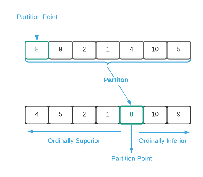
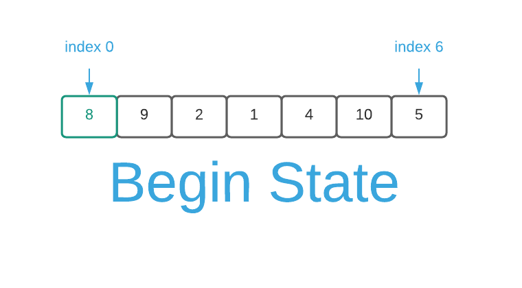
partition accepts a list of data. The item located at index 0 becomes the partition point, also known as the pivot³. In a nut shell, it moves ordinally superior values in front of the pivot and ordinally inferior values after it⁴. The image below depicts a partition operation on a list of integers with a desired ascending sort order.

The important notion here is that partition does not fully sort the data. It provides three guarantees:

1. The partition point is in it’s correct position (the same position as if the data were fully sorted)
2. All items to the left of the partition point are ordinally superior
3. All items to the right of the partition pointer are ordinally inferior

The implementation of partition is vital to the performance of the overall algorithm. Many sources employ an inefficient double loop, similar to insertion sort, due to it’s cognitive simplicity⁵. However, the only way to ensure that the overall asymptotic complexity of the algorithm conforms to the desired $O(n \log_2 n)$ (on average) runtime is to ensure that partition is linear ($O(n)$). Examine the pseudo code in conjunction with the animation below to understand how to properly implement partition.

There is still one important detail that has been ignored to this point, that is the choosePivot method as shown in lines 40 thru 42 of the pseudo code. That is the topic of the next subsection.

Choose Pivot

The purpose of choosePivot is to identify the value in which to partition around. Lines 5 and 6 of the pseudo code describe its use. Removing those two lines has no effect on the end state. This begs the question, why use it? The answer is that it ensures a consistent runtime regardless of the ordering of the input data. This is a bit difficult to comprehend without examples.

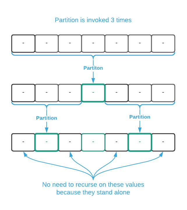
First, consider the ideal scenario where the pivot element is always the median value as depicted below⁶. The asymptotic complexity is better than $O(n \log_2 n)$ in this case. As proof, first note that $n = 7$ meaning there are 7 elements in the list of data. Plugging $n$ into the runtime yields $O(7 \log_2 7) \approx O(20)$. So, the assertion is that the total number of operations is less than 20. partition is involved 3 times: once with 7 elements and twice with 3 elements. Assuming that partition is linear, that’s a total of 13 operations which validates the assertion.

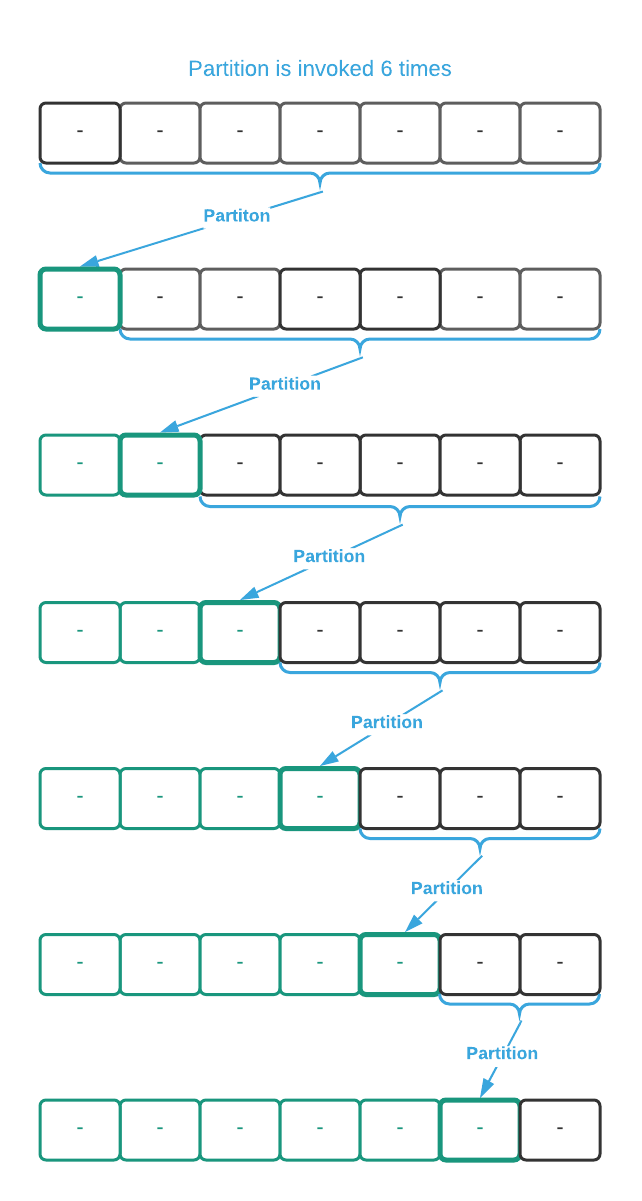
Now consider the other end of the spectrum where the pivot element is always the most ordinally superior value. Using the image below as a guide, partition is involved six times with input sizes of 7, 6, 5, 4, 3, and 2 for a total of 27 operations. That’s more than twice the number of operations in the previous example.

The next question becomes, is it possible to divine the median value? The answer is, unfortunately, no⁷. Determining the median is more computationally intensive than an inefficient sort. One solution is to partition on the first value (index 0). This is equivalent to removing lines 5 and 6 from the pseudo code. This works just as well as any other strategy if the input data is randomly ordered. The problem is that pre-sorted data results in the worst case scenario. Likewise, partitioning on last value (index $n-1$) has the same effect. Choosing the pivot element at random, as shown in the pseudo code, ensures an acceptable runtime regardless of the input data. In fact, it’s proven to result in a $O(n \log_2 n)$ runtime on average⁸.

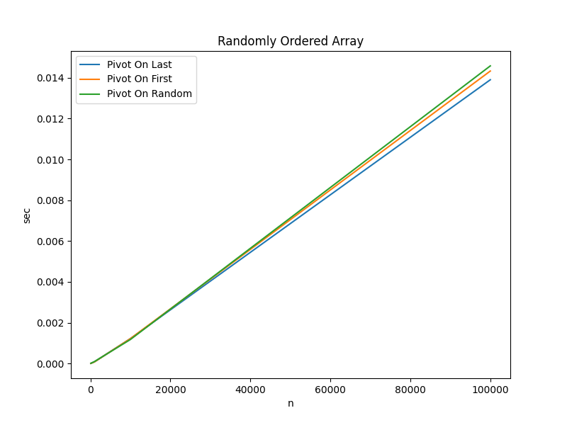
To make this concept a bit more concrete, the data below compares the actual runtimes⁹ for sorting data with the following pivot strategies.

• Pivot on Last: choosePivot returns $n-1$
• Pivot on First: choosePivot returns $0$
• Pivot on Random: choosePivot as depicted in the pseudo code

Randomly Ordered Input Data

Key Takeaways:

• When the input data is randomly ordered, the choice of pivot is inconsequential

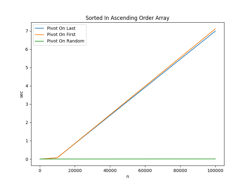
Input Data Sorted in Ascending Order

Key Takeaways:

• When the input data is pre-sorted, selecting the pivot randomly is close to 1,500 times faster
• The random pivot strategy is actually slightly more efficient with pre-sorted data because partitions require fewer swaps

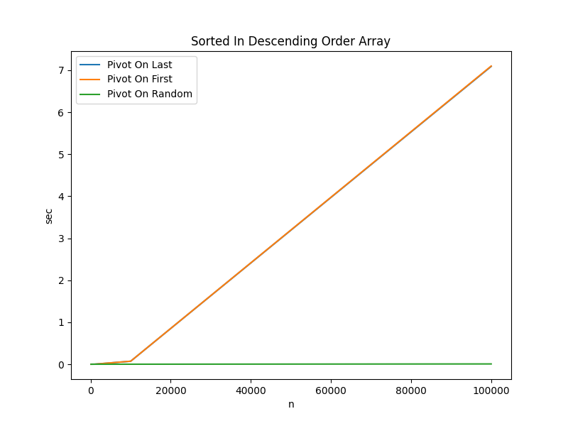
Input Data Sorted in Descending Order

Key Takeaways:

• The results for data sorted in descending order are similar to the results for data sorted in ascending order

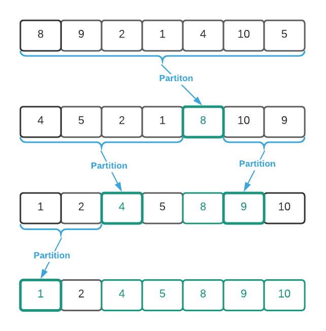
Wrapping it Up

To bring this all together, the image below illustrates sorting a list of integers in ascending order using the quick sort algorithm. For the sake of brevity, it always pivots on the first item (index 0). Because the input data is randomly ordered, this isn’t detrimental to performance.

Pseudo Code

\begin{algorithm}
\caption{Quick Sort}
\begin{algorithmic}
\REQUIRE $A$ = list of numbers
\REQUIRE $n$ = number of items to consider
\ENSURE $A$ sorted in sequential order
\FUNCTION{quickSort}{A, n}
    \IF{$n \leq 1$}
        \RETURN
    \ENDIF
    \STATE pivot $\gets$ \CALL{choosePivot}{n}
    \STATE swap $A_0$ and $A_{\text{pivot}}$
    \STATE pivot $\gets$ \CALL{partition}{A}
    \STATE
    \STATE \CALL{quickSort}{$A_0...A_{\text{pivot - 1}}$, pivot}
    \STATE pivot $\gets$ pivot + 1
    \STATE \CALL{quickSort}{$A_{\text{pivot}}...A_{\text{n-pivot-1}}$, n - pivot}
\ENDFUNCTION
\STATE
\REQUIRE $A$ = list of numbers where $A_0$ is the value to partition around
\ENSURE All values $\lt A_0$ arranged before $A_0$ and values $\gt A_0$ arranged after $A_0$
\OUTPUT position of the value at $A_0$ after the partition
\FUNCTION{partition}{A}
    \STATE low $\gets$ 1
    \STATE high $\gets \vert A \vert - 1$
    \STATE
    \WHILE{true}
        \WHILE{low $\lt$ high and $A_{\text{low}} \lt A_0$}
            \STATE low $\gets$ low + 1
        \ENDWHILE
        \STATE
        \WHILE{high $\geq$ low and $A_{\text{high}} \geq A_0$}
            \STATE high $\gets$ high - 1
        \ENDWHILE
        \STATE
        \IF{low $\geq$ high}
            \BREAK
        \ENDIF
        \STATE
        \STATE swap $A_{\text{low}}$ and $A_{\text{high}}$
        \STATE low $\gets$ low + 1
        \STATE high $\gets$ high - 1
    \ENDWHILE
    \STATE
    \STATE swap $A_0$ and $A_{\text{high}}$
    \RETURN{high}
\ENDFUNCTION
\STATE
\REQUIRE $n$ = number of elements in the partition
\OUTPUT ideal index to partition on
\FUNCTION{choosePivot}{n}
    \RETURN uniformly random number between 0 and $n$ inclusive
\ENDFUNCTION
\end{algorithmic}
\end{algorithm}

Implementation Details

Notice lines 9 and 11 of the pseudo code. Essentially, what’s happening is a recursion on a portion of the input array. In many languages such as Python and ES6, it’s easy to create a slice of an array. For instance, line 9 may be written as follows:

quickSort(A, n):
    ...
    quickSort(A[:pivot - 1], pivot)
    ...

function quickSort(A, n) {
    ...
    quickSort(A.slice(0, pivot - 1), pivot)
    ...
}

There is a glaring problem with this approach. Creating a slice allocates a shallow copy of the array which is wasteful and has negative performance implications. A better approach is recurse on the existing array and specify the start and end index as follows:

quickSort(A, start, end):
    ...
    quickSort(A, start, pivot - 1)
    ...

function quickSort(A, start, end) {
    ...
    quickSort(A, start, pivot - 1)
    ...
}

Asymptotic Complexity

$O(n^2)$; however, it’s $O(n \log_2 n)$ on average

Source Code

Full Repo

Relevant Files:

• quick_sort.h
• quick_sort.c
• quick_sort_test.c

Click here for build and run instructions

Exercises

1. What is the asymptotic memory consumption of the quick sort algorithm?
   Answers (click to expand)

   Both answers are acceptable

   • $\Theta(1)$ - Quick sort is an in place sorting algorithm meaning that it sorts by swapping items within the given list. Therefore, the only additional memory required is the temporary variable used during a swap. - Strictly speaking, this answer is only partially correct; however, it’s acceptable given that this source does not cover stack memory usage with recursive algorithms.
   • $O(\log_2 n)$ - Quick sort is a recursive algorithm so, assuming a non-tail call optimized language, the stack grows with each recursive call.

2. What is the result of removing lines 32 and 33 from the pseudo code considering:
   a. the end state
   b. runtime

   Answers (click to expand)

   1. The change has no effect on the end state of the data. It will continue to sort correctly.
   2. The loop starting at line 18 will suffer two superfluous comparison operations as lines 19 and 23 will evaluate to true at least once.

3. Using the programming language of your choice, implement a quick sort function that accepts:
   • an array of any type
   • a sorting strategy
   • a choose pivot strategy
   Answers (click to expand)

   See the C implementation provided in the links below. Your implementation may vary significantly and still be correct.
   - quick_sort.h
   - quick_sort.c
   - quick_sort_test.c

4. Instrument your quick sort function from the previous exercise to calculate the total number of copy and comparison operations. Next, sort the data contained in the sort.txt file and determine the total number of copy and comparison operations using a “pivot on first (index 0)” strategy.

   Answers (click to expand)

   See the C implementation provided in sort_implementation.c Your implementation may vary significantly and still be correct. The final output should be:

   Quick Sort: copy = 113,769 comparisons = 171,705 total = 285,474
   

   As a reference, here is how quick sort stacks up against the other sorting algorithms.

       Bubble Sort: copy = 71,844,390 comparisons = 49,988,559 total = 121,832,949
    Insertion Sort: copy = 23,968,128 comparisons = 23,958,117 total =  47,926,245
    Selection Sort: copy =     29,964 comparisons = 49,995,000 total =  50,024,964
        Merge Sort: copy =    133,616 comparisons =    120,473 total =     254,089
        Quick Sort: copy =    113,769 comparisons =    171,705 total =     285,474