Running Median

graph LR
	ALG(["fas:fa-trophy Running Median fas:fa-trophy #160;"])

	ASY_ANA(["fas:fa-check Asymptotic Analysis #160;"])
    click ASY_ANA "./math-asymptotic-analysis"

	PQ(["fas:fa-check Priority Queue #160;"])
    click PQ "./data-struct-priority-queue"

    QS(["fas:fa-check Quick Select #160;"])
    click QS "./algorithms-quick-select"

	ASY_ANA-->ALG
	PQ-->ALG
	QS-->ALG

It’s common to combine existing algorithms and data structures together to create new behavior. Running median, aka moving median or median maintenance, is a prime example. The problem is easily solved by repurposing one of the previously covered data structures. As you read through the problem definition below, try to identify the data structure in question before examining the final algorithm.

History

The exact origin of the running median algorithm as applied to computing may be lost to the annals of time or, at the very least, it’s difficult to ascertain. It seems as if nearly every algorithms textbook contains a non-attributed version. A close cousin of running median is running average and its use dates back as early as 1901¹. The original purpose was to smooth erratic data for statistical analysis.

Consider a scenario where you need to repeatedly calculate the median² value from a stream of numbers as shown below.

There are a few ways to tackle the problem. For instance, one might maintain a sort order and find the median via direct addressing as shown in the pseudo code below.

\begin{algorithm}
\caption{Running Median using a sorted array}
\begin{algorithmic}
\REQUIRE A = list of values
\REQUIRE value = value to add to A
\OUTPUT median value in $A \cup \text{value}$
\FUNCTION{runningMedian}{A, value}
    \STATE A $\gets A \cup \text{value}$
    \STATE A $\gets$ \CALL{sort}{A}
    \STATE $n \gets \vert A \vert$
    \STATE mid $\gets \floor{\frac{n}{2}}$
    \IF{$n \bmod 2 = 0$}
        \RETURN $\frac{A_{\text{mid}} + A_{\text{mid} - 1}}{2}$
    \ENDIF
    \RETURN $A_{\text{mid}}$
\ENDFUNCTION
\STATE
\FUNCTION{main}{}
    \STATE A $\gets \emptyset$ 
    \STATE \CALL{runningMedian}{A, 10}
    \STATE \CALL{runningMedian}{A, 5}
    \STATE \CALL{runningMedian}{A, 15}
    \STATE \CALL{runningMedian}{A, 20}
    \STATE \CALL{runningMedian}{A, 1}
    \STATE \CALL{runningMedian}{A, 17}
\ENDFUNCTION
\end{algorithmic}
\end{algorithm}

This is an effective solution; however, it is limited by the speed of the sort function. Recall from the sorting section that the lower limit for a comparison based sort algorithm is $O(n \log_2{n})$. Capitalizing on the fact that the data is largely pre-sorted could bring the sort runtime down to $O(n)$ on average. Therefore, it’s safe to assume that the asymptotic complexity of this solution is $O(n)$ on average³.

Astute readers will no doubt realize that this is similar to quick select. This algorithm is a viable option to obviate sorting. See the pseudo code below.

\begin{algorithm}
\caption{Running Median using quick select}
\begin{algorithmic}
\REQUIRE A = list of values
\REQUIRE value = value to add to A
\OUTPUT median value in $A \cup \text{value}$
\FUNCTION{runningMedian}{A, value}
    \STATE A $\gets A \cup \text{value}$
    \STATE $n \gets \vert A \vert$
    \STATE mid $\gets \floor{\frac{n}{2}}$
    \IF{$n \bmod 2 = 0$}
        \STATE first-value $\gets$ \CALL{quickSelect}{A, mid}
        \STATE second-value $\gets$ \CALL{quickSelect}{A, mid - 1}
        \RETURN $\frac{\text{first-value} + \text{second-value}}{2}$
    \ENDIF
    \RETURN \CALL{quickSelect}{A, mid}
\ENDFUNCTION
\STATE
\FUNCTION{main}{}
    \STATE A $\gets \emptyset$ 
    \STATE \CALL{runningMedian}{A, 10}
    \STATE \CALL{runningMedian}{A, 5}
    \STATE \CALL{runningMedian}{A, 15}
    \STATE \CALL{runningMedian}{A, 20}
    \STATE \CALL{runningMedian}{A, 1}
    \STATE \CALL{runningMedian}{A, 17}
\ENDFUNCTION
\end{algorithmic}
\end{algorithm}

The quick select version of the algorithm yields slightly better actual run times. However, it’s still essentially a $O(n \log_2{n})$ algorithm that runs in $O(n)$ time on average. Reiterating the question in the opening paragraph, what data structure can be leveraged to create a superior solution? The answer is priority queue, aka heap.

As review, a priority queue tracks a list of items and returns either the minimum or maximum value, as defined by a priority function, in constant ($\Theta(1)$) time. Furthermore, insert operations are $O(\log_2 n)$. The trick is figuring out how to get a priority queue to track a median value. The reader is encouraged to contemplate this before forging ahead.

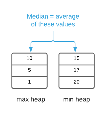
It’s not possible for a single heap to track a median value; however, it is possible using two. If half the values are in a minimum heap and the other half are in a maximum heap, the top of the heaps will always hold the median values. To be clear, the minimum heap’s priority function prioritizes smaller values and the maximum heap’s priority function prioritizes larger values. For example, the image below depicts the list $\{10, 5, 15, 20, 1, 17\}$ using this technique.

The running median algorithm is dependant on three invariants:

1. When the total count of items is even, each heap has an equal number of items (see image above)
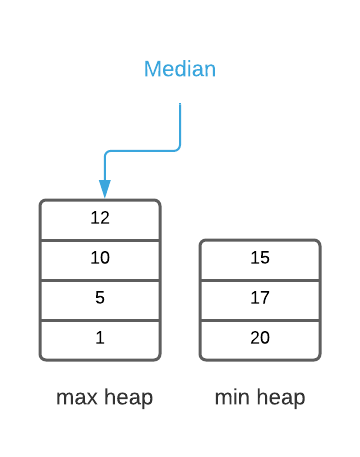
2. When the total count of items is odd, one heap has exactly one more item than the other (see the image below)
3. All of the values in the maximum heap are smaller than the values in the minimum heap

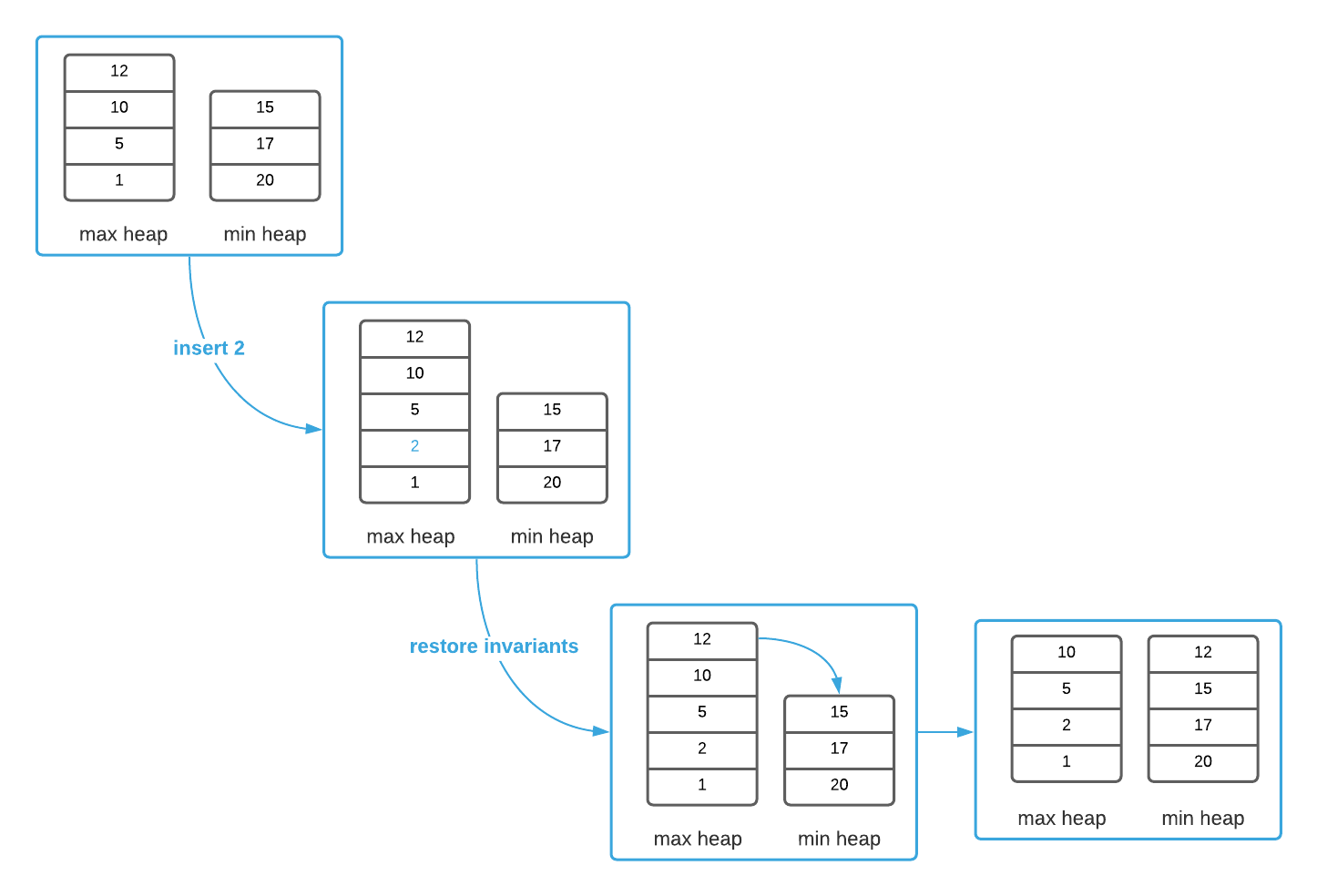
It’s necessary to restore the invariants after each insert operation. This often entails removing an item from one heap and placing it in the other as the image below illustrates.

In the worst case, inserting a new value entails 3 $O(\log_2{n})$ queue operations. One to insert the initial value, one to remove an item from a heap, and a final one to insert the value into the appropriate heap. Calculating the median is a constant ($\Theta(1)$) operation as the salient values are readily available at the top of the heaps. The overall runtime reduces to $O(\log_2{n})$. That’s an impressive improvement. Study the pseudo code to see the final product.

Applications

• Removing anomalies from time series with minimal impact on the overall data as is common in financial and economic data analysis
• Filters to smooth erratic sensor data

Pseudo Code

\begin{algorithm}
\caption{Running Median using priority queues}
\begin{algorithmic}
\REQUIRE min-heap, max-heap
\REQUIRE value = value to append
\OUTPUT median value of all invocations
\FUNCTION{runningMedian}{min-heap, max-heap, value}
    \IF{value $\leq$ \CALL{heapPeek}{min-heap}}
        \STATE \CALL{heapInsert}{min-heap}{value}
    \ELSE
        \STATE \CALL{heapInsert}{max-heap}{value}
    \ENDIF
    \STATE
    \STATE \CALL{balanceHeaps}{min-heap, max-heap}
    \STATE
    \STATE n $\gets$ \CALL{heapSize}{min-heap} + \CALL{heapSize}{max-heap}
    \IF{$n \bmod 2 = 0$}
        \STATE first-value $\gets$ \CALL{heapPeek}{min-heap}
        \STATE second-value $\gets$ \CALL{heapPeek}{max-heap}
        \RETURN $\frac{\text{first-value} + \text{second-value}}{2}$
    \ELSE
        \IF{\CALL{heapSize}{min-heap} $\gt$ \CALL{heapSize}{max-heap}}
            \RETURN \CALL{heapPeek}{min-heap}
        \ELSE
            \RETURN \CALL{heapPeek}{max-heap}
        \ENDIF
    \ENDIF
\ENDFUNCTION
\STATE
\REQUIRE min-heap, max-heap
\ENSURE if n is even, min-heap 
\FUNCTION{balanceHeaps}{min-heap, max-heap}
    \WHILE{\CALL{isBalanced}{min-heap, max-heap} = FALSE}
        \IF{\CALL{heapSize}{min-heap} $\gt$ \CALL{heapSize}{max-heap}}
            \STATE \CALL{heapInsert}{max-heap, \CALL{heapExtract}{min-heap}}
        \ELSE
            \STATE \CALL{heapInsert}{min-heap, \CALL{heapExtract}{max-heap}}
        \ENDIF
    \ENDWHILE
\ENDFUNCTION
\STATE
\REQUIRE min-heap, max-heap
\OUTPUT true if heaps are balanced and false otherwise
\FUNCTION{isBalanced}{min-heap, max-heap}
    \STATE min-heap-size $\gets$ \CALL{heapSize}{min-heap}
    \STATE max-heap-size $\gets$ \CALL{heapSize}{max-heap}
    \STATE n $\gets$ min-heap-size + max-heap-size
    \STATE
    \IF{$n \bmod 2 = 0$}
        \RETURN min-heap-size = max-heap-size
    \ELSE
        \RETURN $\abs{\text{min-heap-size} - \text{max-heap-size}} = 1$
    \ENDIF
\ENDFUNCTION
\end{algorithmic}
\end{algorithm}

Asymptotic Complexity

• Median: $O(1)$
• Insert: $O(\log_{2}n)$

Source Code

Full Repo

Relevant Files:

• running_median.h
• running_median.c
• running_median_test.c

Click here for build and run instructions

Exercises

1. Assuming that performance is your primary concern, suppose you have an array of 100,000 randomly sorted integers and you need to determine the median value contained therein. Which algorithm, running median or quick select, is best suited for this use case. Explain your answer.

   Answers (click to expand)

   Quick select is a best suited to this use case. Because the array is static, quick select can divine the median using 2 $O(n)$ operations (see the "Running Median using quick select" pseudo code).
   
   Running median requires inserting each value into a heap at a cost of $O(\log_2{n})$ per insert. Therfore, the overall complexity is $O(n \log_2{n})$.

2. Using the programming language of your choice, implement the running median algorithm.

   Answers (click to expand)

   See the C implementation provided in the links below. Your implementation may vary significantly and still be correct.
   - running_median.h
   - running_median.c
   - running_median_test.c

3. The random_floating_points.txt file contains 100,000 floating point numbers. Feed the numbers into your running median algorithm one at a time and sum the results. The logic should be similar to the following:

    sum = 0
    for each value in random_floating_points.txt:
        sum += RunningMedian(value)
    return sum
   

   Answers (click to expand)

   See the C implementation provided in the SumOfMedians function located in this file: running_median_test_case.c. Your implementation may vary significantly and still be correct. The final output should be: 4995738.755804.

4. Without changing the asymptotic complexity of your running median algorithm, modify it to return the median of the last 100 values. To clarify, suppose you invoke your running median function 101 times. The first 100 invocations behave as before. The 101^th invocation should exclude the value from the first invocation in the median calculation. For bonus points, allow the consumer to specify the size of the sliding window.

   HINT: You will need to make use of another data structure and add delete functionality to your heap implementation.

   Answers (click to expand)

   See the C implementation provided in the links below. Your implementation may vary significantly and still be correct.
   - running_median.h
   - running_median.c
   - running_median_test.c
   See the pseudo code solution here.

5. Complete exercise 3 again using the modified algorithm you created for exercise 4.

   Answers (click to expand)

   See the C implementation provided in the SumOfMedians function located in this file: running_median_test_case.c. Your implementation may vary significantly and still be correct. The final output should be: 4995205.397700.