The Knapsack Problem

The knapsack problem is without a doubt a “must know” for any software professional. Wikipedia reports that “out of 75 algorithmic problems, the knapsack problem [is] the 19^th most popular and the third most needed”¹. Regardless of your particular domain, it’s highly probable that you will need to understand this algorithm’s particulars.

Suppose you have a number of items of varying size and value that you need to place inside a knapsack. Unfortunately, the knapsack isn’t large enough to hold all the items. You need a strategy for packing the knapsack with items that have the highest possible total value. Stated in computer science terms, you have $2n+1$ positive integers². $n$ is the number of items. Each item has an associated value ($v_i$) and size ($s_i$). The final integer is the capacity ($C$) of the knapsack. This algorithm will select the subset of items with a total size lower than $C$ ($\sum_{i \in S} s_i \leq C$) that also has the maximum possible total value ($\max{\sum_{i \in S} v_i}$). This is best demonstrated with an example. Consider the image below.

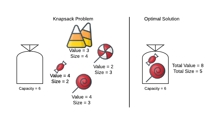
Consider the knapsack a convenient abstraction. This is a useful algorithm for any scenario where a scarce resource must be managed optimally.

Now that the concept of the Knapsack problem is clear, it’s time deliver some bad news: it is in $NP$-hard. However, there are many tractable approaches beyond brute-force search.

1. Dynamic Programming: The demonstrated algorithm runs in $O(nC)$ where $n$ is the number of items and $C$ is the knapsack capacity. There are two caveats. The first is that $C$ and each $s$ must be a discrete number (the pseudo code should make it clear why). The second is that the runtime becomes prohibitive for large values of $C$.

   The knapsack problem is $NP$-hard and this section demonstrates a non-approximated polynomial time solution. It is time to collect the million dollars and live turkey³? Not quite… The run time quoted above is actually pseudo-polynomial, meaning that it’s polynomial in relation to the numeric value of the input; however, it’s exponential in relation to the input’s length (size in bits). Every order of magnitude increase to the numeric value of $C$ (increase in input length by 1 bit) results in exponentially more loops. Algorithms such as this one are said to be weakly $NP$-hard.

Applications

• Internet download managers - Cargo loading
• Production scheduling
• Capital budgeting
• Portfolio management

Asymptotic Complexity

• Dynamic Programming: $O(nC)$ where $n$ is the number of items and $C$ is the knapsack capacity.

Pseudo Code

Dynamic Programming

inputs:
    S = array of sizes
    V = array of values
    C = capacity of knapsack
    n = number of items

knapsack:
    solutions[n + 1][C + 1]

    for i = 0 to C:
        solutions[0][i] = 0;

    for i = 1 to n + 1:
        for c = 0 to C + 1:
            if S[i] < c:
                solutions[i][c] = solutions[i - 1][c]
            else if solutions[i - 1][c] > solutions[i - 1][S[i] + V[i]:
                solutions[i][c] = solutions[i - 1][c]
            else
                solutions[i][c] = solutions[i - 1][S[i] + V[i]

    return solustions[n][C];

Source Code

Full Repo

Relevant Files:

• KnapsackProblem.h
• KnapsackProblem.c
• KnapsackProblemTests.c

Click here for build and run instructions