Prerequisites (click to view)
graph LR
	ALG(["fas:fa-trophy Strassen Matrix Multiplication fas:fa-trophy #160;"])

	ASY_ANA(["fas:fa-check Asymptotic Analysis #160;"])
    click ASY_ANA "./math-asymptotic-analysis"

	ARRAY(["fas:fa-check Array #160;"])
    click ARRAY "./list-data-struct-array"

	MAT(["fas:fa-check Matrices #160;"])
    click MAT "./math-matrices"

	MAT-->ALG
	ASY_ANA-->ALG
	ARRAY-->ALG
Matrices are a computing staple and the quest to squeeze every last drop of efficiency from related algorithms is never ending. They are the basic building blocks - as well as the “bottleneck” - of computer graphics and data science1 applications. Due to their fundamental nature, even a meager increase in performance would advance state of the art in many different fields including: artificial intelligence, machine learning, simulation, and visualization.
The latest advancements in matrix manipulation aren’t really algorithmic; rather, they are driven by specialized hardware. The highly parallelized nature of GPUs (Graphics Processing Units) and FPGAs (Field Programmable Gate Array) make them ideally suited for the task. Unfortunately, hardware is outside of the scope of this work. That does not however imply that the study of matrix manipulation is not worthwhile. It is an ideal scholastic device. The algorithms make heavy use of nested loops and repeated memory access which are ubiquitous programming mechanisms. The most important concepts introduced here are general optimization techniques that apply to all algorithms.
As a survey of the topic, five different matrix multiplication algorithms are explored below. The first four are all $\Theta(n^3)$; however, they have considerably different execution times. The final one is the ingenious Strassen matrix multiplication algorithm which is $\Theta(n^{2.81})$. For the sake of brevity, this material makes the simplifying assumption that all matrices are perfect squares and the size is a power of two (e.g. $2 \times 2, 4 \times 4, 8 \times 8, 16 \times 16,…$). Intrigued readers are encouraged to modify the algorithms to accept any size of matrix as an independent study project.
History
Volker Strassen shocked the computing world when he published his eponymous matrix multiplication algorithm in 19692. At that point, it was widely accepted that $\Theta(n^3)$ was a hard limit that couldn’t be improved on. Strassen’s work decimated this illusion and inspired a plethora of follow on research. The theoretical lower bound has yet to be conclusively proven.
It’s typical to represent matrices as 2-dimensional arrays3; therefore, it is the approach employed here. It’s recommended that readers quickly review the Array section; specifically, the Direct Addressing, Multi-Dimensional Arrays, and Spatial Locality subsections. All of those concepts are vital to this section. As a final note, the Matrices pre-requisite provides a quick primer on the mathematical concepts contained here.
Naive Matrix Multiply
It’s always a good idea to start with the simplest possible solution. See the naive algorithm shown below.
\begin{algorithm}
\caption{Naive Matrix Multiplication}
\begin{algorithmic}
\REQUIRE $n$ = size of the matrices
\REQUIRE $A,B$ = $n \times n$ matrices
\OUTPUT $A * B$
\FUNCTION{naiveMatrixMultiply}{$n,A,B$}
	\STATE $C \gets n \times n$ matrix
    \FOR{$i \gets 0$ to $n-1$}
		\FOR{$j \gets 0$ to $n-1$}
            \FOR{$k \gets 0$ to $n-1$}
				\STATE $C_{i,j} = C_{i,j} + A_{i,k} * B_{k,j}$
			\ENDFOR
		\ENDFOR
	\ENDFOR
	\RETURN $C$
\ENDFUNCTION
\end{algorithmic}
\end{algorithm}
If you have a performance problem, the first step is always to create some benchmarks4. The table below outlines the benchmarks for multiplying random matrices of size $n$5.
| Algorithm | n=16 | n=32 | n=64 | n=128 | n=256 | n=512 |
|---|---|---|---|---|---|---|
| Naive Matrix Multiply | 0.000005 sec | 0.000032 sec | 0.000331 sec | 0.002320 sec | 0.033331 sec | 0.266140 sec |
The algorithm can multiply a $512 \times 512$ matrix in $\approx$ 266 milliseconds. That may or may not be sufficient depending on the application. For the purposes here, we’ll assume that it does not meet our needs. Based on the fact that this is an $\Theta(n^3)$ algorithm, one can make some predictions. Specifically, doubling the input size should increase the runtime by a factor of eight. For instance:
\[n=16 \quad 16^3 = 4096\\ 4096 * 8 = 32768\\ n=32 \quad 32^3 = 32768 \\\]With numbers as small as those shown above, there is bound to be a great deal of noise. However, the prediction is generally validated by the data. A matrix of size $128 \times 128$ executed in 0.033331 seconds and a matrix of size $512 \times 512$ took 0.266140 seconds.
\[\frac{0.266140}{0.033331} \approx 7.98\]Is it therefore reasonable to assume that a matrix of size $1024 \times 1024$ will execute in $\approx$ 2.13 seconds? See the benchmarks for larger matrices below to find out.
| Algorithm | n=1024 | n=2048 |
|---|---|---|
| Naive Matrix Multiply | 6.835343 sec | 93.427716 sec |
One might be surprised to find that a matrix of size $1024 \times 1024$ ran $\approx$ 25 times slower than a matrix of size $512 \times 512$. Obviously, there is something more than meets the eye. The problem here is spatial locality6. Notice that line 6 of the pseudo code is accessing $B$ in column-row order rather than the more efficient row-column order. The next algorithm attempts to address this problem.
Tiling Matrix Multiply
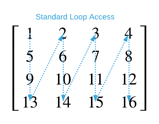
Loop tiling is a common remedy to cache miss problems. The general idea is to break a loop into smaller sub iterations in order to minimize cache misses. This is difficult to visualize without an example. Consider the simple column-row loop below.
\begin{algorithm}
\caption{Standard Matrix Loop}
\begin{algorithmic}
\REQUIRE $n$ = size of the matrices
\REQUIRE $A$ = $n \times n$ matrix
\FUNCTION{standardLoop}{$n,A$}
    \FOR{$i \gets 0$ to $n-1$}
		\FOR{$j \gets 0$ to $n-1$}
            \STATE $A_{j,i}$ \COMMENT{do something with this value}
		\ENDFOR
	\ENDFOR
\ENDFUNCTION
\end{algorithmic}
\end{algorithm}
The result is the following matrix access pattern.

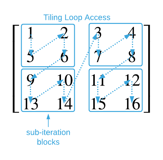
Contrast the standard loop with a tiling loop.
\begin{algorithm}
\caption{Tiling Matrix Loop}
\begin{algorithmic}
\REQUIRE $n$ = size of the matrices
\REQUIRE $A$ = $n \times n$ matrix
\FUNCTION{tilingLoop}{$n,A$}
    \STATE block-size = 2
    \WHILE{ii $\lt$ n}
        \WHILE{jj $\lt$ n}
            \FOR{$i \gets ii$ to min(n, ii + block-size)}
                \FOR{$j \gets jj$ to min(n, jj + block-size)}
                    \STATE $A_{j,i}$ \COMMENT{do something with this value}
                \ENDFOR
            \ENDFOR
             \STATE jj $\gets$ jj + block-size
         \ENDWHILE
         \STATE ii $\gets$ ii + block-size
     \ENDWHILE
\ENDFUNCTION
\end{algorithmic}
\end{algorithm}
The tiling loop generates the access pattern depicted below.

The tiling version of the matrix multiplication algorithm is shown below.
\begin{algorithm}
\caption{Tiling Matrix Multiplication}
\begin{algorithmic}
\REQUIRE $n$ = size of the matrices
\REQUIRE $A$ = $n \times n$ matrix
\FUNCTION{tilingLoop}{$n,A$}
    \STATE block-size = 16 \COMMENT{tune this value for your platform}
	\STATE $C \gets n \times n$ matrix
    \WHILE{ii $\lt$ n}
        \WHILE{jj $\lt$ n}
            \WHILE{kk $\lt$ n}
                \FOR{$i \gets ii$ to min(n, ii + block-size)}
                    \FOR{$j \gets jj$ to min(n, jj + block-size)}
                        \FOR{$k \gets kk$ to min(n, kk + block-size)}
                            \STATE $C_{i,j} = C_{i,j} + A_{i,k} * B_{k,j}$
                        \ENDFOR
                    \ENDFOR
                \ENDFOR
                 \STATE kk $\gets$ kk + block-size
             \ENDWHILE
             \STATE jj $\gets$ jj + block-size
         \ENDWHILE
         \STATE ii $\gets$ ii + block-size
     \ENDWHILE
\ENDFUNCTION
\end{algorithmic}
\end{algorithm}
Now it’s time to compare benchmarks to verify the cache miss theory.
| Algorithm | n=16 | n=32 | n=64 | n=128 | n=256 | n=512 |
|---|---|---|---|---|---|---|
| Naive Matrix Multiply | 0.000005 sec | 0.000032 sec | 0.000331 sec | 0.002320 sec | 0.033331 sec | 0.266140 sec |
| Tiling Matrix Multiply | 0.000007 sec | 0.000065 sec | 0.000416 sec | 0.002957 sec | 0.019936 sec | 0.170470 sec |
For matrices of size $128 \times 128$ and smaller the new tiling algorithm is slightly less performant. This is to be expected because the extra loops are not free; they required processor cycles. However, larger matrices fair much better due to fewer cache misses. Notice the benchmarks for larger matrices below.
| Algorithm | n=1024 | n=2048 |
|---|---|---|
| Naive Matrix Multiply | 6.835343 sec | 93.427716 sec |
| Tiling Matrix Multiply | 1.484321 sec | 17.959455 sec |
Tiling is $\approx$ 5 times faster than the naive algorithm for matrices of size $1024 \times 1024$ and larger. That’s an impressive improvement! However, the $\approx$ 18 seconds for a matrix of size $2048 \times 2048$ is still unacceptable. We’ve successfully reduced cache misses but we created extra work in the process.
Transpose Matrix Multiply
The problem with the previous two algorithms is that they access the first matrix in row-column order and the second in column-row order. The goal is to access both matrices in row-column order. A simple way to achieve this is to simply transpose one of the matrices as shown in the pseudo code below.
\begin{algorithm}
\caption{Transpose Matrix Multiplication}
\begin{algorithmic}
\REQUIRE $n$ = size of the matrices
\REQUIRE $A,B$ = $n \times n$ matrices
\OUTPUT $A * B$
\FUNCTION{transposeMatrixMultiply}{$n,A,B$}
	\STATE $C \gets n \times n$ matrix
    \STATE $D \gets B^T$
    \FOR{$i \gets 0$ to $n-1$}
		\FOR{$j \gets 0$ to $n-1$}
            \FOR{$k \gets 0$ to $n-1$}
				\STATE $C_{i,j} = C_{i,j} + A_{i,k} * D_{j,k}$
			\ENDFOR
		\ENDFOR
	\ENDFOR
	\RETURN $C$
\ENDFUNCTION
\end{algorithmic}
\end{algorithm}
The updated benchmarks are shown below.
| Algorithm | n=16 | n=32 | n=64 | n=128 | n=256 | n=512 |
|---|---|---|---|---|---|---|
| Tiling Matrix Multiply | 0.000007 sec | 0.000065 sec | 0.000416 sec | 0.002957 sec | 0.019936 sec | 0.170470 sec |
| Transpose Matrix Multiply | 0.000008 sec | 0.000095 sec | 0.000569 sec | 0.003368 sec | 0.022738 sec | 0.187665 sec |
The cost of transposing the second matrix is considerable and it equates to slightly higher execution times for matrices of $512 \times 512$ and smaller. However, larger matrices show improvements as shown in the benchmarks below.
| Algorithm | n=1024 | n=2048 |
|---|---|---|
| Tiling Matrix Multiply | 1.484321 sec | 17.959455 sec |
| Transpose Matrix Multiply | 1.459802 sec | 11.990165 sec |
For a $2048 \times 2048$ matrix, the transpose algorithm saves $\approx$ 6 seconds which is notable but the runtime is still not acceptable.
Recursive Matrix Multiply
Notice that the naive multiplication algorithm outperforms all the others for small matrices. The goal of this algorithm is to capitalize on this by reducing large matrix operations to several operations on smaller matrices. Astute readers will recognize this as another implementation of the Divide and Conquer design paradigm.
\begin{algorithm}
\caption{Recursive Matrix Multiplication}
\begin{algorithmic}
\REQUIRE $n$ = size of the matrices where $n$ is a power of 2 (4, 8, 16, 32,...)
\REQUIRE $A,B$ = $n \times n$ matrices
\OUTPUT $A * B$
\FUNCTION{recursiveMatrixMultiply}{$n,A,B$}
    \IF{$n \leq 16$} \COMMENT{tune this value for your platform}
        \RETURN \CALL{naiveMatrixMultiplication}{n, A, B}
    \ENDIF
    \STATE \COMMENT{Split the matrices into sub-matrices that are $\frac{1}{4}$ the size of the original}
    \STATE $\begin{bmatrix} A_1 & A_2 \\ A_3 & A_4 \end{bmatrix} \gets \text{submatrices of} \; A$
    \STATE $\begin{bmatrix} B_1 & B_2 \\ B_3 & B_4 \end{bmatrix} \gets \text{submatrices of} \; B$
    \STATE
    \STATE $Q_1$ = \CALL{recursiveMatrixMultiply}{$\frac{n}{2}, A_1, B_1$} + \CALL{recursiveMatrixMultiply}{$\frac{n}{2}, A_2, B_3$}
    \STATE $Q_2$ = \CALL{recursiveMatrixMultiply}{$\frac{n}{2}, A_1, B_2$} + \CALL{recursiveMatrixMultiply}{$\frac{n}{2}, A_2, B_4$}
    \STATE $Q_3$ = \CALL{recursiveMatrixMultiply}{$\frac{n}{2}, A_3, B_1$} + \CALL{recursiveMatrixMultiply}{$\frac{n}{2}, A_4, B_3$}
    \STATE $Q_4$ = \CALL{recursiveMatrixMultiply}{$\frac{n}{2}, A_3, B_2$} + \CALL{recursiveMatrixMultiply}{$\frac{n}{2}, A_4, B_4$}
    \STATE \RETURN $\begin{bmatrix} Q_1 & Q_2 \\ Q_3 & Q_4 \end{bmatrix}$
\ENDFUNCTION
\end{algorithmic}
\end{algorithm}
One obvious down side of this approach is all the extra copy operations. Each recursion allocates new memory for sub-matrices. On the plus side, each smaller matrix is optimally sized to reduce cache misses. The benchmarks tell the full story.
| Algorithm | n=16 | n=32 | n=64 | n=128 | n=256 | n=512 |
|---|---|---|---|---|---|---|
| Transpose Matrix Multiply | 0.000008 sec | 0.000095 sec | 0.000569 sec | 0.003368 sec | 0.022738 sec | 0.187665 sec |
| Recursive Matrix Multiply | 0.000006 sec | 0.000049 sec | 0.000442 sec | 0.002447 sec | 0.019743 sec | 0.151945 sec |
| Algorithm | n=1024 | n=2048 |
|---|---|---|
| Transpose Matrix Multiply | 1.459802 sec | 11.990165 sec |
| Recursive Matrix Multiply | 1.155591 sec | 9.507868 sec |
The recursive algorithm yields a small performance gain across the board. The final algorithm aims to further improve execution times by reducing recursions.
Strassen Matrix Multiply
Notice that the recursive matrix multiplication algorithm spawns eight new recursions for each recursive call. The Strassen algorithm, through what can only be described as genius, reduces the new recursions from eight to seven. That’s a 12.5% recurse reduction. Study the pseudo code below to gain an appreciation of the algorithm.
\begin{algorithm}
\caption{Strassen Matrix Multiplication}
\begin{algorithmic}
\REQUIRE $n$ = size of the matrices where $n$ is a power of 2 (4, 8, 16, 32,...)
\REQUIRE $A,B$ = $n \times n$ matrices
\OUTPUT $A * B$
\FUNCTION{strassenMatrixMultiply}{$n,A,B$}
    \IF{$n \leq 16$} \COMMENT{tune this value for your platform}
        \RETURN \CALL{naiveMatrixMultiplication}{n, A, B}
    \ENDIF
    \STATE \COMMENT{Split the matrices into sub-matrices that are $\frac{1}{4}$ the size of the original}
    \STATE $\begin{bmatrix} A_1 & A_2 \\ A_3 & A_4 \end{bmatrix} \gets \text{submatrices of} \; A$
    \STATE $\begin{bmatrix} B_1 & B_2 \\ B_3 & B_4 \end{bmatrix} \gets \text{submatrices of} \; B$
    \STATE
    \STATE $P_1 \gets$ \CALL{strassenMatrixMultiply}{$\frac{n}{2}, A_1, B_2 - B_4$}
    \STATE $P_2 \gets$ \CALL{strassenMatrixMultiply}{$\frac{n}{2}, A_1 + A_2, B_4$}
    \STATE $P_3 \gets$ \CALL{strassenMatrixMultiply}{$\frac{n}{2}, A_3 + A_4, B_1$}
    \STATE $P_4 \gets$ \CALL{strassenMatrixMultiply}{$\frac{n}{2}, A_4, B_3 - B_1$}
    \STATE $P_5 \gets$ \CALL{strassenMatrixMultiply}{$\frac{n}{2}, A_1 + A_4, B_1 + B_4$}
    \STATE $P_6 \gets$ \CALL{strassenMatrixMultiply}{$\frac{n}{2}, A_2 - A_4, B_3 + B_4$}
    \STATE $P_7 \gets$ \CALL{strassenMatrixMultiply}{$\frac{n}{2}, A_1 - A_3, B_1 + B_2$}
    \RETURN $\begin{bmatrix} P_5+P_4−P_2+P_6 & P_1+P_2 \\ P_3 + P_4 & P_1+P_5-P_3−P_7 \end{bmatrix}$
\ENDFUNCTION
\end{algorithmic}
\end{algorithm}
The first obvious observation is that this algorithm has a good deal of overhead in the form of extra matrix addition and subtraction operations. It’s difficult to make a meaningful performance prediction by examining the pseudo code. This is an all-to-common conundrum and it speaks to the importance of benchmarking. Luckily, we’ve been collecting data throughout this performance improvement effort.
| Algorithm | n=16 | n=32 | n=64 | n=128 | n=256 | n=512 |
|---|---|---|---|---|---|---|
| Recursive Matrix Multiply | 0.000006 sec | 0.000049 sec | 0.000442 sec | 0.002447 sec | 0.019743 sec | 0.151945 sec |
| Strassen Matrix Multiply | 0.000005 sec | 0.000071 sec | 0.000361 sec | 0.002306 sec | 0.015871 sec | 0.097818 sec |
Examining the data above reveals a modest performance improvement for small matrices.
| Algorithm | n=1024 | n=2048 |
|---|---|---|
| Recursive Matrix Multiply | 1.155591 sec | 9.507868 sec |
| Strassen Matrix Multiply | 0.764536 sec | 4.995162 sec |
For large matrices, the gains are more impressive. The execution time for matrices of size $2048 \times 2048$ realized close to a 50% reduction. Recall that the naive algorithm took $\approx$ 93 seconds: Strassen is $\approx$ 19 times faster.
While there are still plenty of performance improvements to be made; unfortunately, this is as far as this material is going to go. There is easily an entire book of content solely on this subject. Consider this section a short primer to the topic. As alluded to in the beginning, the purpose of this piece is not to teach matrix multiplication. Rather, it’s to endow the reader with a few tools to employ in their performance improvement endeavors.
Actual Run Times
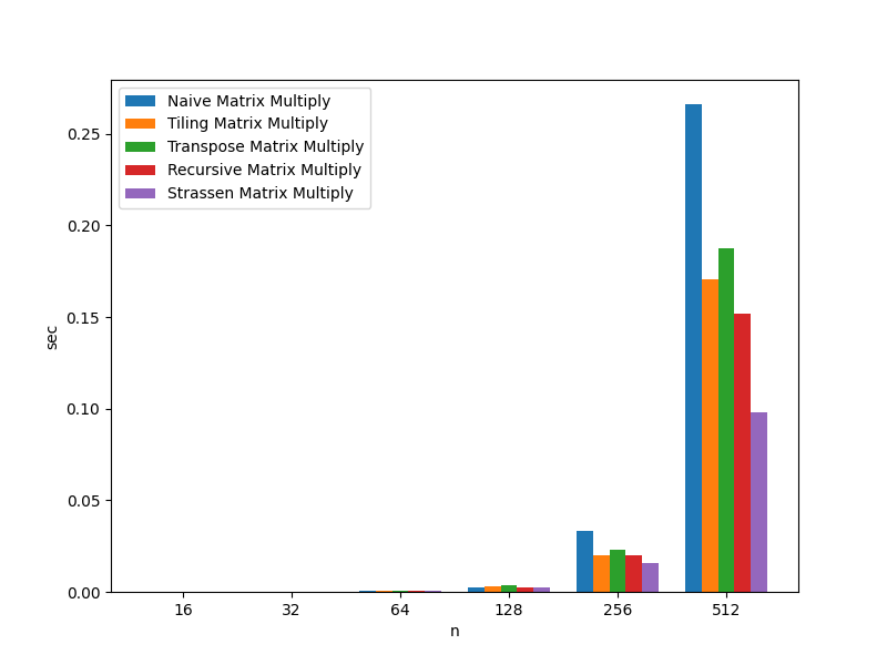
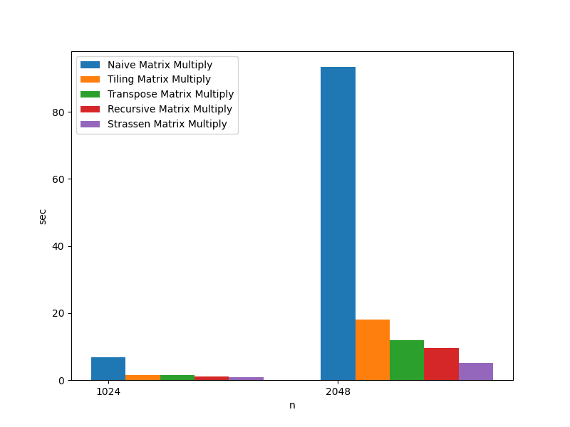
For convenience, the benchmark data presented throughout this section is compiled here. The charts and tables below outlines the benchmarks for multiplying random matrices of size $n$5.

| Algorithm | n=16 | n=32 | n=64 | n=128 | n=256 | n=512 |
|---|---|---|---|---|---|---|
| Naive Matrix Multiply | 0.000005 sec | 0.000032 sec | 0.000331 sec | 0.002320 sec | 0.033331 sec | 0.266140 sec |
| Tiling Matrix Multiply | 0.000007 sec | 0.000065 sec | 0.000416 sec | 0.002957 sec | 0.019936 sec | 0.170470 sec |
| Transpose Matrix Multiply | 0.000008 sec | 0.000095 sec | 0.000569 sec | 0.003368 sec | 0.022738 sec | 0.187665 sec |
| Recursive Matrix Multiply | 0.000006 sec | 0.000049 sec | 0.000442 sec | 0.002447 sec | 0.019743 sec | 0.151945 sec |
| Strassen Matrix Multiply | 0.000005 sec | 0.000071 sec | 0.000361 sec | 0.002306 sec | 0.015871 sec | 0.097818 sec |

| Algorithm | n=1024 | n=2048 |
|---|---|---|
| Naive Matrix Multiply | 6.835343 sec | 93.427716 sec |
| Tiling Matrix Multiply | 1.484321 sec | 17.959455 sec |
| Transpose Matrix Multiply | 1.459802 sec | 11.990165 sec |
| Recursive Matrix Multiply | 1.155591 sec | 9.507868 sec |
| Strassen Matrix Multiply | 0.764536 sec | 4.995162 sec |
Applications
- Modern data science is built largely upon linear algebra which makes heavy use of matrices
- Graph theory
- Physics engines
- Finance
- Graphics
Pseudo Code
For convenience, all the algorithms shown above are repeated here.
\begin{algorithm}
\caption{Naive Matrix Multiplication}
\begin{algorithmic}
\REQUIRE $n$ = size of the matrices
\REQUIRE $A,B$ = $n \times n$ matrices
\OUTPUT $A * B$
\FUNCTION{naiveMatrixMultiply}{$n,A,B$}
	\STATE $C \gets n \times n$ matrix
    \FOR{$i \gets 0$ to $n-1$}
		\FOR{$j \gets 0$ to $n-1$}
            \FOR{$k \gets 0$ to $n-1$}
				\STATE $C_{i,j} = C_{i,j} + A_{i,k} * B_{k,j}$
			\ENDFOR
		\ENDFOR
	\ENDFOR
	\RETURN $C$
\ENDFUNCTION
\end{algorithmic}
\end{algorithm}
\begin{algorithm}
\caption{Tiling Matrix Multiplication}
\begin{algorithmic}
\REQUIRE $n$ = size of the matrices
\REQUIRE $A$ = $n \times n$ matrix
\FUNCTION{tilingLoop}{$n,A$}
    \STATE block-size = 16 \COMMENT{tune this value for your platform}
	\STATE $C \gets n \times n$ matrix
    \WHILE{ii $\lt$ n}
        \WHILE{jj $\lt$ n}
            \WHILE{kk $\lt$ n}
                \FOR{$i \gets ii$ to min(n, ii + block-size)}
                    \FOR{$j \gets jj$ to min(n, jj + block-size)}
                        \FOR{$k \gets kk$ to min(n, kk + block-size)}
                            \STATE $C_{i,j} = C_{i,j} + A_{i,k} * B_{k,j}$
                        \ENDFOR
                    \ENDFOR
                \ENDFOR
                 \STATE kk $\gets$ kk + block-size
             \ENDWHILE
             \STATE jj $\gets$ jj + block-size
         \ENDWHILE
         \STATE ii $\gets$ ii + block-size
     \ENDWHILE
\ENDFUNCTION
\end{algorithmic}
\end{algorithm}
\begin{algorithm}
\caption{Transpose Matrix Multiplication}
\begin{algorithmic}
\REQUIRE $n$ = size of the matrices
\REQUIRE $A,B$ = $n \times n$ matrices
\OUTPUT $A * B$
\FUNCTION{transposeMatrixMultiply}{$n,A,B$}
	\STATE $C \gets n \times n$ matrix
    \STATE $D \gets B^T$
    \FOR{$i \gets 0$ to $n-1$}
		\FOR{$j \gets 0$ to $n-1$}
            \FOR{$k \gets 0$ to $n-1$}
				\STATE $C_{i,j} = C_{i,j} + A_{i,k} * D_{j,k}$
			\ENDFOR
		\ENDFOR
	\ENDFOR
	\RETURN $C$
\ENDFUNCTION
\end{algorithmic}
\end{algorithm}
\begin{algorithm}
\caption{Recursive Matrix Multiplication}
\begin{algorithmic}
\REQUIRE $n$ = size of the matrices where $n$ is a power of 2 (4, 8, 16, 32,...)
\REQUIRE $A,B$ = $n \times n$ matrices
\OUTPUT $A * B$
\FUNCTION{recursiveMatrixMultiply}{$n,A,B$}
    \IF{$n \leq 16$} \COMMENT{tune this value for your platform}
        \RETURN \CALL{naiveMatrixMultiplication}{n, A, B}
    \ENDIF
    \STATE \COMMENT{Split the matrices into sub-matrices that are $\frac{1}{4}$ the size of the original}
    \STATE $\begin{bmatrix} A_1 & A_2 \\ A_3 & A_4 \end{bmatrix} \gets \text{submatrices of} \; A$
    \STATE $\begin{bmatrix} B_1 & B_2 \\ B_3 & B_4 \end{bmatrix} \gets \text{submatrices of} \; B$
    \STATE
    \STATE $Q_1$ = \CALL{recursiveMatrixMultiply}{$\frac{n}{2}, A_1, B_1$} + \CALL{recursiveMatrixMultiply}{$\frac{n}{2}, A_2, B_3$}
    \STATE $Q_2$ = \CALL{recursiveMatrixMultiply}{$\frac{n}{2}, A_1, B_2$} + \CALL{recursiveMatrixMultiply}{$\frac{n}{2}, A_2, B_4$}
    \STATE $Q_3$ = \CALL{recursiveMatrixMultiply}{$\frac{n}{2}, A_3, B_1$} + \CALL{recursiveMatrixMultiply}{$\frac{n}{2}, A_4, B_3$}
    \STATE $Q_4$ = \CALL{recursiveMatrixMultiply}{$\frac{n}{2}, A_3, B_2$} + \CALL{recursiveMatrixMultiply}{$\frac{n}{2}, A_4, B_4$}
    \STATE \RETURN $\begin{bmatrix} Q_1 & Q_2 \\ Q_3 & Q_4 \end{bmatrix}$
\ENDFUNCTION
\end{algorithmic}
\end{algorithm}
\begin{algorithm}
\caption{Strassen Matrix Multiplication}
\begin{algorithmic}
\REQUIRE $n$ = size of the matrices where $n$ is a power of 2 (4, 8, 16, 32,...)
\REQUIRE $A,B$ = $n \times n$ matrices
\OUTPUT $A * B$
\FUNCTION{strassenMatrixMultiply}{$n,A,B$}
    \IF{$n \leq 16$} \COMMENT{tune this value for your platform}
        \RETURN \CALL{naiveMatrixMultiplication}{n, A, B}
    \ENDIF
    \STATE \COMMENT{Split the matrices into sub-matrices that are $\frac{1}{4}$ the size of the original}
    \STATE $\begin{bmatrix} A_1 & A_2 \\ A_3 & A_4 \end{bmatrix} \gets \text{submatrices of} \; A$
    \STATE $\begin{bmatrix} B_1 & B_2 \\ B_3 & B_4 \end{bmatrix} \gets \text{submatrices of} \; B$
    \STATE
    \STATE $P_1 \gets$ \CALL{strassenMatrixMultiply}{$\frac{n}{2}, A_1, B_2 - B_4$}
    \STATE $P_2 \gets$ \CALL{strassenMatrixMultiply}{$\frac{n}{2}, A_1 + A_2, B_4$}
    \STATE $P_3 \gets$ \CALL{strassenMatrixMultiply}{$\frac{n}{2}, A_3 + A_4, B_1$}
    \STATE $P_4 \gets$ \CALL{strassenMatrixMultiply}{$\frac{n}{2}, A_4, B_3 - B_1$}
    \STATE $P_5 \gets$ \CALL{strassenMatrixMultiply}{$\frac{n}{2}, A_1 + A_4, B_1 + B_4$}
    \STATE $P_6 \gets$ \CALL{strassenMatrixMultiply}{$\frac{n}{2}, A_2 - A_4, B_3 + B_4$}
    \STATE $P_7 \gets$ \CALL{strassenMatrixMultiply}{$\frac{n}{2}, A_1 - A_3, B_1 + B_2$}
    \RETURN $\begin{bmatrix} P_5+P_4−P_2+P_6 & P_1+P_2 \\ P_3 + P_4 & P_1+P_5-P_3−P_7 \end{bmatrix}$
\ENDFUNCTION
\end{algorithmic}
\end{algorithm}
Asymptotic Complexity
- Naive Matrix Multiplication - $\Theta(n^3)$
- Tiling Matrix Multiplication - $\Theta(n^3)$
- Transpose Matrix Multiplication - $\Theta(n^3)$
- Recursive Matrix Multiplication - $\Theta(n^3)$
- Strassen Matrix Multiplication - $\Theta(n^{2.81})$
Source Code
Relevant Files:
Click here for build and run instructions
Exercises
-
Answer each of the following questions with True or False
a. It’s never advisable to use the Naive Matrix Multiplication algorithm.
b. The Strassen Matrix Multiplication algorithm is the state-of-the-art in matrix multiplication.
c. Spatial Locality has a profound impact on matrix multiplication.Answers (click to expand)
- False - For small matrices, the naive algorithm is the best performer.
- False - Matrix multiplication is a complex topic that's beyond the scope of this work. This is a mere primer.
- True - The first four algorithms are all $\Theta(n^3)$; however, they have significantly different execution times because some of them make more efficient use of memory caching.
-
Using the programming language of your choice, implement the Strassen matrix multiplication algorithm.
Answers (click to expand)
See the C implementation provided in the links below. Your implementation may vary significantly and still be correct.
- matrix_operations.h
- matrix_operations.c
- matrix_operations_test.c -
The random_matrix_1.txt and random_matrix_2.txt text files define two matrices of size $4096 \times 4096$ that are comprised of random values between 0 and 100. Each line in the file represents a matrix row formatted as:
{value}<tab>{value}<tab>{value}<tab>...
Using the Strassen matrix multiplication algorithm created for the previous exercise, multiplyrandom_matrix_1.txtbyrandom_matrix_2.txt. Finally, sum each individual value in the resulting matrix. As an example:
\(\begin{bmatrix} 1 & 2 \\ 3 & 4 \end{bmatrix} \times \begin{bmatrix} 5 & 6 \\ 7 & 8 \end{bmatrix} \quad = \quad \begin{bmatrix} 19 & 22 \\ 43 & 50 \end{bmatrix} \quad = \quad 19 + 22 + 43 + 50 \quad = \quad \blueci{134}\)Answers (click to expand)
See the
Cimplementation provided in theMultiplyLargeMatraciesfunction located in this file: matrix_operation_test_case.c. Your implementation may vary significantly and still be correct. The final output should be:
168,345,695,003,062
For reference, theCimplementation completed the task in $\approx$ 40 seconds running on a Surface Book 2 Laptop (Intel Core i7, 16 GB RAM).
-
Linear algebra, which is built upon matrices, is at the heart of modern data science. ↩
-
Available online at https://link.springer.com/article/10.1007/BF02165411 ↩
-
To be 100% accurate, many programming languages with multidimensional array primitives use Iliffe vectors rather than standard C style arrays. This can significantly change the runtime behavior of these algorithms. Regardless, the concepts presented here are still valid. ↩
-
This seems fairly obvious, but it’s all-too-common to skip this step in practice. Failure to generate benchmarks almost always leads to a black hole of wasted time and superfluous effort. It’s analogous to trying to navigate a jungle without a map. Learn from the pain of those who came before and don’t neglect this step. ↩
-
Results will vary depending on the hardware and current workload of the machine on which the benchmarks are run. All data was collected using a docker container running on a Surface Book 2 Laptop (Intel Core i7, 16 GB RAM). ↩ ↩2
-
The exact matrix size that will produce this behavior is highly dependant on the on CPU architecture so don’t be surprised if your results differ significantly. ↩