Prerequisites (click to view)
graph LR
	ALG(["fas:fa-trophy Head-to-Head Comparison fas:fa-trophy #160;"])

	ASY_ANA(["fas:fa-check Asymptotic Analysis #160;"])
    click ASY_ANA "./math-asymptotic-analysis"

	ARRAY(["fas:fa-check Array #160;"])
    click ARRAY "./list-data-struct-array"

	SORTED_ARRAY(["fas:fa-check Sorted Array #160;"])
    click SORTED_ARRAY "./list-data-struct-sorted-array"

	BT(["fas:fa-check Binary Tree #160;"])
    click BT "./list-data-struct-binary-tree"

	SBT(["fas:fa-check Self Balancing Binary Tree #160;"])
    click SBT "./list-data-struct-self-bal-tree"

	RBT(["fas:fa-check Red-Black Tree #160;"])
    click RBT "./list-data-struct-red-black-tree"

	LL(["fas:fa-check Linked List #160;"])
    click LL "./list-data-struct-linked-list"

	ASY_ANA-->ALG
    ARRAY-->SORTED_ARRAY-->ALG
    LL-->ALG
    BT-->SBT-->RBT-->ALG
Recall from this chapter’s introduction that a visceral conception of list data structures is a must for anyone wishing to excel in the software field. The vast majority of software requires tracking a collection of objects in some form or another. The choice of list data structure has a significant impact on both utility and performance. Furthermore, a through understand of popular list tracking patterns is invaluable in the event that one must design their own collection.
In order to solidify your understanding, it’s helpful to compare and contrast list data structures at a high level. The table below details the asymptotic complex of common operations.
| Operation | Array | Sorted Array | Linked List | Binary Tree | Red-Black Tree |
|---|---|---|---|---|---|
| Direct Address | $O(1)$ | $O(1)$ | N/A | N/A | N/A |
| Insert | $O(n)$ | $O(n)$ | $O(1)$ | $O(height)$ | $O(\log_{2}n)$ |
| Delete | $O(n)$ | $O(n)$ | $O(1)$ | $O(height)$ | $O(\log_{2}n)$ |
| Search | $O(n)$ | $O(\log_2{n})$ | $O(n)$ | $O(height)$ | $O(\log_{2}n)$ |
| Enumerate | $\Theta(n)$ | $\Theta(n)$ | $\Theta(n)$ | $\Theta(n + height)$ | $\Theta(n + \log_{2}n)$ |
| Min | $\Theta(n)$ | $O(1)$ | $\Theta(n)$ | $O(height)$ | $O(\log_{2}n)$ |
| Max | $\Theta(n)$ | $O(1)$ | $\Theta(n)$ | $O(height)$ | $O(\log_{2}n)$ |
| Predecessor | $\Theta(n)$ | $O(1)$ | $\Theta(n)$ | $O(height)$ | $O(\log_{2}n)$ |
| Successor | $\Theta(n)$ | $O(1)$ | $\Theta(n)$ | $O(height)$ | $O(\log_{2}n)$ |
| Rank | $\Theta(n)$ | $O(1)$ | $\Theta(n)$ | $O(height)$ | $O(\log_{2}n)$ |
Recall from Real World Asymptotic Complexity that asymptotic complexity is a single part of a larger whole. The following section is meant to provide concrete evidence of such.
Actual Run Times
Often times, academia has little deference for real-world application. This section aims to avoid such a blunder by providing actual run times1. The reader is encouraged to experiment by re-producing the data below on their own machine, making modifications, and examining the results. Instructions for generating run time data are available in the Actual Run Times section of the Source Code page.
As a word of caution, an unhealthy preoccupation with performance is a common malady. Consider the data below for what it is: data. The reader has the responsibly to transform it into information applicable to a particular context. Always refer back to the principle of parsimony as a balancing force. The best data structure for your application is the simplest one that satisfies your requirements (one of which may be performance).
The charts and accompanying tables below outline the actual run times for n
operations on various data structures of size n. In the case that a particular
operation has a symmetric counterpart2, the counterpart is omitted as
results would lack sufficient variation to be deemed interesting. The data
includes seven variations of list data structures, five of which are implemented
exactly as described in the material.
The remaining two list data structures are special cases constructed to demonstrate salient concepts.
- Linked List Poor Locality: A linked list with suboptimal spatial locality. Constituent items are located at least 10,000 bytes apart in memory. Although not shown, the same scenario is possible with binary trees.
- Binary Tree Unbalanced: A binary search tree where all items are inserted in sequential order. If necessary, consult Self Balancing Binary Tree for a refresher.
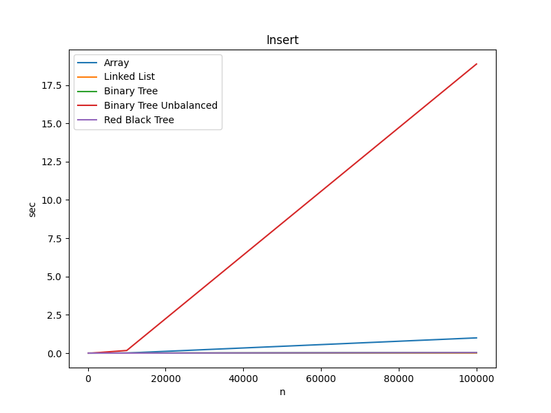
Insert
| Structure | n=100 | n=1000 | n=10000 | n=100000 |
|---|---|---|---|---|
| Array | 0.000015 sec | 0.000079 sec | 0.006310 sec | 0.994912 sec |
| Linked List | 0.000005 sec | 0.000034 sec | 0.000343 sec | 0.003312 sec |
| Binary Tree | 0.000007 sec | 0.000104 sec | 0.001770 sec | 0.035700 sec |
| Binary Tree Unbalanced | 0.000015 sec | 0.002076 sec | 0.171654 sec | 18.873086 sec |
| Red Black Tree | 0.000010 sec | 0.000118 sec | 0.001766 sec | 0.036463 sec |
Key Takeaways:
- Inserting 100,000 items into an Array is approximately 1 second slower than inserting the same items into a Linked list.
- Inserting 100,000 items in sequential order into a Binary Tree takes close to 19 seconds.
- For a small number of items, Binary Trees are slightly more performant than Red-Black Trees. However, with 100,000 items Red-Black Tree inserts become slightly more performant because of balancing. In reality, this is an academically interesting result but the difference is insignificant.
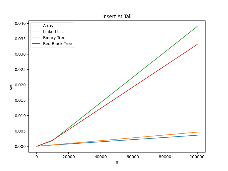
In data above, the new item is inserted at the head of the Array. Inserting an item at the tail of an Array may be dramatically faster (possibly even faster than linked lists) depending on the language and the contents of memory. To demonstrate, the data below was collected while inserting the new item at the tail of the array.
| Structure | n=100 | n=1000 | n=10000 | n=100000 |
|---|---|---|---|---|
| Array | 0.000010 sec | 0.000043 sec | 0.000372 sec | 0.003573 sec |
| Linked List | 0.000005 sec | 0.000039 sec | 0.000436 sec | 0.004576 sec |
| Binary Tree | 0.000008 sec | 0.000105 sec | 0.001814 sec | 0.038957 sec |
| Red Black Tree | 0.000011 sec | 0.000134 sec | 0.001919 sec | 0.033101 sec |
Key Takeaways:
- Inserting an item at the tail of an Array is dramatically faster than inserting an item at the head. While a reallocation is still required, the items do not need to be rearranged in memory.
Search
| Structure | n=100 | n=1000 | n=10000 | n=100000 |
|---|---|---|---|---|
| Array | 0.000021 sec | 0.001893 sec | 0.192644 sec | 20.135746 sec |
| Sorted Array | 0.000003 sec | 0.000029 sec | 0.000443 sec | 0.004700 sec |
| Linked List | 0.000014 sec | 0.001237 sec | 0.116017 sec | 13.677152 sec |
| Linked List Poor Locality | 0.000026 sec | 0.006498 sec | 1.389610 sec | 384.067171 sec |
| Binary Tree | 0.000010 sec | 0.000135 sec | 0.002325 sec | 0.028518 sec |
| Binary Tree Unbalanced | 0.000050 sec | 0.005280 sec | 0.520024 sec | 51.581549 sec |
| Red Black Tree | 0.000003 sec | 0.000053 sec | 0.001037 sec | 0.019234 sec |
Key Takeaways:
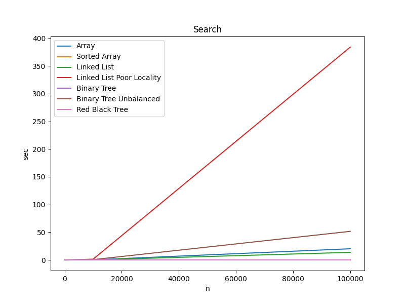
- Searching a Sorted Array, Binary Tree, or Red-Black Tree is lighting fast.
- 100,000 search operations on a randomly sorted Array is more than 20 seconds slower than 100,000 search operations on a Sorted Array.
- Search operations on an Unbalanced Binary Tree are painfully slow.
- A Linked List with suboptimal spatial locality has the worst performance by far and demonstrates the implications of not being able to take advantage of the cache. Repeatedly accessing memory that is not stored contiguously causes cache misses, which are expensive.
Enumerate
| Structure | n=100 | n=1000 | n=10000 | n=100000 |
|---|---|---|---|---|
| Array | 0.000001 sec | 0.000001 sec | 0.000003 sec | 0.000027 sec |
| Sorted Array | 0.000000 sec | 0.000001 sec | 0.000004 sec | 0.000028 sec |
| Linked List | 0.000001 sec | 0.000002 sec | 0.000019 sec | 0.000193 sec |
| Linked List Poor Locality | 0.000001 sec | 0.000005 sec | 0.000104 sec | 0.002054 sec |
| Binary Tree | 0.000002 sec | 0.000015 sec | 0.000186 sec | 0.001583 sec |
| Binary Tree Unbalanced | 0.000001 sec | 0.000005 sec | 0.000039 sec | 0.000363 sec |
| Red Black Tree | 0.000001 sec | 0.000007 sec | 0.000087 sec | 0.000964 sec |
Key Takeaways:
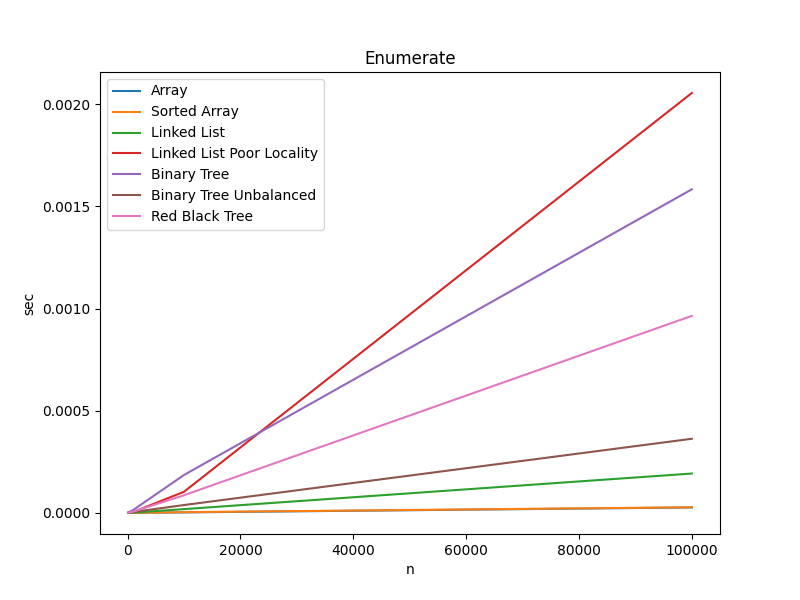
- There is less than .002 seconds difference between each data structure over 100,000 items.
Max
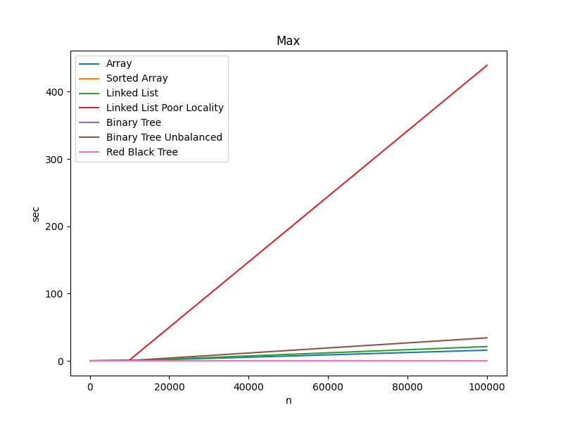
| Structure | n=100 | n=1000 | n=10000 | n=100000 |
|---|---|---|---|---|
| Array | 0.000016 sec | 0.001698 sec | 0.157349 sec | 15.782043 sec |
| Sorted Array | 0.000001 sec | 0.000002 sec | 0.000013 sec | 0.000130 sec |
| Linked List | 0.000020 sec | 0.002133 sec | 0.222554 sec | 21.181374 sec |
| Linked List Poor Locality | 0.000020 sec | 0.004259 sec | 1.084074 sec | 439.200296 sec |
| Binary Tree | 0.000002 sec | 0.000008 sec | 0.000064 sec | 0.000391 sec |
| Binary Tree Unbalanced | 0.000012 sec | 0.003264 sec | 0.349664 sec | 34.142476 sec |
| Red Black Tree | 0.000001 sec | 0.000006 sec | 0.000157 sec | 0.001691 sec |
Key Takeaways:
- When there are 10,000 or fewer items in a collection, the choice of data structure is close to inconsequential.
- Finding the Max value in a large Array or Linked List is unreasonably slow.
- A Linked List with suboptimal spatial locality has dire performance implications.
Predecessor
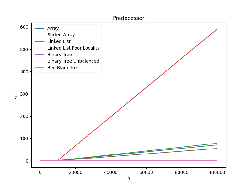
| Structure | n=100 | n=1000 | n=10000 | n=100000 |
|---|---|---|---|---|
| Array | 0.000056 sec | 0.005415 sec | 0.592855 sec | 71.003978 sec |
| Sorted Array | 0.000003 sec | 0.000033 sec | 0.000435 sec | 0.005575 sec |
| Linked List | 0.000086 sec | 0.008289 sec | 0.812207 sec | 78.459917 sec |
| Linked List Poor Locality | 0.000077 sec | 0.007699 sec | 1.579743 sec | 589.928713 sec |
| Binary Tree | 0.000005 sec | 0.000047 sec | 0.000965 sec | 0.007140 sec |
| Binary Tree Unbalanced | 0.000054 sec | 0.005520 sec | 0.522937 sec | 54.988196 sec |
| Red Black Tree | 0.000002 sec | 0.000044 sec | 0.000392 sec | 0.007062 sec |
Key Takeaways:
- These results highlight the importance of search tree balance.
- Because data was inserted into the Binary Tree in random order, the run times are comparable with Red-Black Tree.
- A Linked List with suboptimal spatial locality has dire performance implications.
Rank
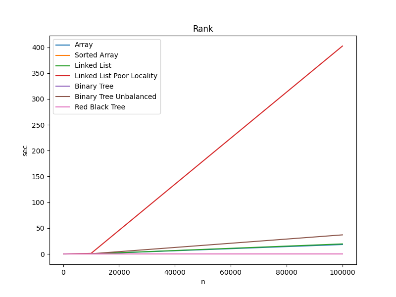
| Structure | n=100 | n=1000 | n=10000 | n=100000 |
|---|---|---|---|---|
| Array | 0.000025 sec | 0.002207 sec | 0.183034 sec | 18.222195 sec |
| Sorted Array | 0.000002 sec | 0.000019 sec | 0.000313 sec | 0.002957 sec |
| Linked List | 0.000017 sec | 0.002251 sec | 0.214607 sec | 19.418371 sec |
| Linked List Poor Locality | 0.000018 sec | 0.005014 sec | 1.078370 sec | 402.518668 sec |
| Binary Tree | 0.000003 sec | 0.000021 sec | 0.000259 sec | 0.002615 sec |
| Binary Tree Unbalanced | 0.000018 sec | 0.003281 sec | 0.349165 sec | 36.926841 sec |
| Red Black Tree | 0.000002 sec | 0.000022 sec | 0.000258 sec | 0.003379 sec |
Key Takeaways:
- Rank, Predecessor, and Max have virtually the same run time results because the algorithms are similar.
Source Code
Relevant Files:
Click here for details on generating actual run time data
Exercises
-
Using the programming language of your choice, code insert, delete, and search, operations for an array, linked list, and binary tree.
PRO TIP: Create a suite of unit tests to validate your list data structure algorithms.
-
Results will vary depending on the hardware and current workload of the machine on which the benchmarks are run. All data was collected using a docker container running on a Surface Book 2 Laptop (Intel Core i7, 16 GB RAM). ↩
-
Insert/Delete, Min/Max, and Predecessor/Successor are all symmetric operations. ↩