Prerequisites (click to view)
graph LR
	ALG(["fas:fa-trophy Closest Pair fas:fa-trophy #160;"])

	ASY_ANA(["fas:fa-check Asymptotic Analysis #160;"])
    click ASY_ANA "./math-asymptotic-analysis"

	GRAPH(["fas:fa-check Graphing #160;"])
    click GRAPH "./math-graphing"

	MS(["fas:fa-check Merge Sort #160;"])
    click MS "./sorting-merge"

	ASY_ANA-->ALG
    GRAPH-->ALG
    MS-->ALG
This section is our first instance of a geometric algorithm, that is, an algorithm intended to translate to the arrangement of objects in an Euclidean space. The graphics, robotics, geography, and simulation fields, to name a few, are all dominated by algorithms of this ilk. The specific problem addressed here is closest pair - given a series of points on a plane, identify the pair of points that are closest together. For pedagogical reasons, we’ll first examine the problem as applied to a one-dimensional space and then we’ll expand the solution to accommodate two dimensions.
History
The closest pair algorithm was first introduced in 1975 in a paper entitled Closest-Point Problems by Michael Ian Shamos and Dan Hoey1. It was the first of many forays into the field of computational complexity as applied to geometric algorithms. This field is more commonly know as computational geometry.
One-Dimension
Assume you have the points $\{-1, 5, 0, -5, 2, -3\}$ and you need to find the two that are closest together. The nuclear option is to compare each point to all the other points as outlined in the pseudo code below. This brute force approach yields a $\Theta(n^2)$ runtime, which makes it suitable for our small use case, but impractical for large data sets.
\begin{algorithm}
\caption{Closest Pair - One Dimension - Brute Force}
\begin{algorithmic}
\REQUIRE $A$ = set points representing coordinates on a plane having $\vert A \vert \geq 2$
\OUTPUT the distance between the two closest points
\FUNCTION{closestPairBruteForce}{A}
    \STATE closest-dist $\gets \infty$
    \STATE
    \FOR{$p1 \in A$}
        \FOR{$p2 \in A$}
            \STATE \COMMENT{$\vert\quad\vert$ denotes absolute value in this instance}
            \IF{$p1 \neq p2$ and $\vert p1 - p2 \vert \lt$ closest-dist}
                \STATE closest-dist = $\vert p1 - p2 \vert$
            \ENDIF
        \ENDFOR
    \ENDFOR
    \STATE
    \RETURN closest-dist
\ENDFUNCTION
\end{algorithmic}
\end{algorithm}
In order to improve the runtime, consider the algorithm from the perspective of geometry. Essentially, what we want to do is lay the points out on a number line and scan for the answer. See the image below.
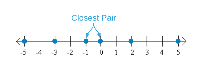
Unfortunately, machines don’t accept an “arrange points on a number line and scan” command. The algorithmic equivalent is sorting and searching. Once the numbers are in order, a single linear scan comparing each point to the previous point yields the answer. Study the pseudo code below to gain an appreciation of the concept. The revised algorithm’s runtime is dominated by the sort operation on line 2. Recall that the lower bound of any sort algorithm is $O(n \log_2{n})$. Lines 5 thru 9 add an additional $\Theta(n)$ of work. $O(n \log_2{n} + n)$ reduces to $O(n \log_2{n})$. That’s a respectable improvement.
\begin{algorithm}
\caption{Closest Pair - One Dimension}
\begin{algorithmic}
\REQUIRE $A$ = set points representing coordinates on a plane having $\vert A \vert \geq 2$
\OUTPUT the distance between the two closest points
\FUNCTION{closestPair}{$A$}
    \STATE $A \gets$ \CALL{sort}{A}
    \STATE closest-dist = $A_1 - A_0$
    \STATE
    \FOR{i $\gets 2$ to $\vert A \vert - 1$}
        \IF{$A_i - A_{i-1} \lt$ closest-dist}
            \STATE closest-dist = $A_{i} - A_{i-1}$
        \ENDIF
    \ENDFOR
    \STATE
    \RETURN closest-dist
\ENDFUNCTION
\end{algorithmic}
\end{algorithm}
The algorithm shown above is the simplest - and likely most performant - means of locating the two closest points on a single-dimensional plane. However, the technique doesn’t translate to the more difficult two-dimensional problem. We’ll apply the divide and conquer paradigm in order to build advanced concepts. Before continuing, try to apply this recipe to the algorithm on your own.
The image below depicts the divide and conquer version of the single-dimensional closest point algorithm. Just like the simpler version above, it is $O(n \log_2{n})$. The first step is sorting the points. Next is the divide portion of the recipe which consists of splitting the data down the middle and finding the closest pairs recursively. The last recipe step, combine, comes with a twist. The closest pairs from the left and right side are known. However, the recursive calculations preclude the distance of the points that span the left and right data cuts. We’ll call this pair the split pair. In the case of the image below, that’s $(-1, 0)$. The overall closest pair is the minimum of the left, right, and split pairs.
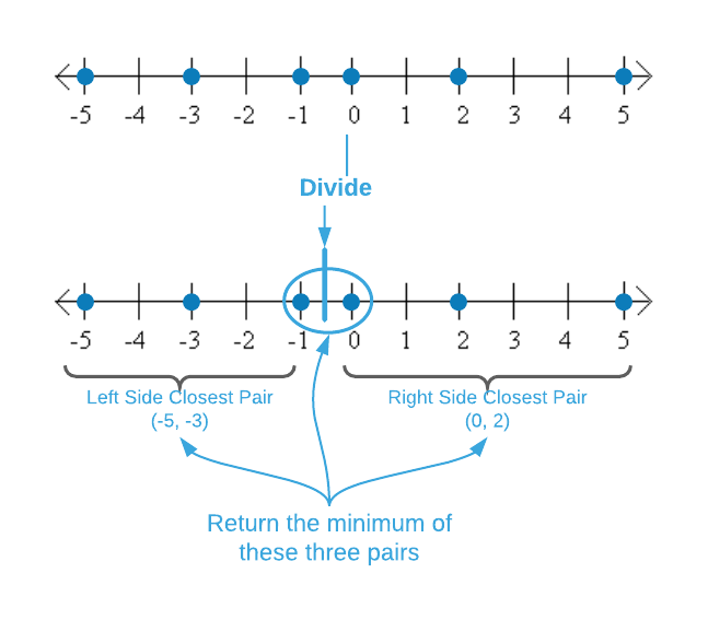
The pseudo code for the algorithm is below. The combine step - finding the minimum of the left, right, and split pairs - is a key concept for the two-dimensional version of the problem. It’s highly recommend that readers implement this algorithm in their language of choice before addressing the next subsection.
\begin{algorithm}
\caption{Closest Pair - One Dimension - Divide and Conquer}
\begin{algorithmic}
\REQUIRE $A$ = set points representing coordinates on a plane having $\vert A \vert \geq 2$
\OUTPUT the distance between the two closest points
\FUNCTION{closestPair}{A}
    \STATE A $\gets$ \CALL{sort}{A}
    \RETURN \CALL{closestPairRecursive}{A}
\ENDFUNCTION
\STATE
\REQUIRE $A$ = set points, sorted in ascending order, representing coordinates on a plane having $\vert A \vert \geq 2$
\OUTPUT the distance between the two closest points
\FUNCTION{closestPairRecursive}{A}
    \STATE n $\gets \vert A \vert$
    \IF{n $\leq$ 3}
        \RETURN \CALL{closestPairBruteForce}{A}
    \ENDIF
    \STATE
    \STATE mid $\gets \floor{\frac{n}{2}}$
    \STATE left-closest-dist $\gets$ \CALL{closestPairRecursive}{$\{A_0...A_{\text{mid} - 1}\}$}
    \STATE right-closest-dist $\gets$ \CALL{closestPairRecursive}{$\{A_{\text{mid}}...A_{n-1}\}$}
    \STATE split-closest-dist $\gets A_{\text{mid}} - A_{\text{mid - 1}}$
    \STATE
    \RETURN \CALL{min}{left-closest-dist, right-closest-dist, split-closest-dist}
\ENDFUNCTION
\end{algorithmic}
\end{algorithm}
Two-Dimensions
The two-dimensional version of the closest pair problem is: given a list of
Cartesian coordinates, identify the pair that has the smallest Euclidean
distance between them. As a quick refresher2, a Cartesian coordinate is
two numbers3 that specify the x and y positions on a 2-dimensional
plane4. For instance, the image below depicts the two coordinate sets
(2, 3) and (-3, -3).
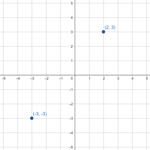
The Euclidean distance calculation is slightly more complex than the one-dimensional case. The formula is:
\[d(p1, p2) = \sqrt{(p2_x - p1_x)^2 + (p2_y - p1_y)^2}\]As an example, calculating the Euclidean distance between the two points shown above yields:
\[p1 = (2, 3)\\ p2 = (-3, -3)\\ d(p1, p2) = \sqrt{(-3 - 2)^2 + (-3 - 3)^2} \approx 7.81\]With the preliminaries out of the way, it’s time to dive right in. Before reading on, devise your own brute force algorithm for the two-dimensional closest distance problem. What are the differences between your algorithm and the single-dimensional brute force algorithm?
There are minimal differences between the one and two-dimensional brute force algorithms as shown in the pseudo code below. In fact, the only dissimilarity is the distance calculation. Both have identical asymptotic complexities ($\Theta(n^2)$).
\begin{algorithm}
\caption{Closest Pair - Two Dimensions - Brute Force}
\begin{algorithmic}
\REQUIRE $A$ = set of 2-tuples representing $x$ and $y$ coordinates on a plane having $\vert A \vert \geq 2$
\OUTPUT the distance between the two closest points as measured by Euclidean distance
\FUNCTION{closestPairBruteForce}{A}
    \STATE closest-dist $\gets$ \CALL{distance}{$A_0$, $A_1$}
    \STATE
    \FOR{$p1 \in A$}
        \FOR{$p2 \in A$}
            \IF{$p1 \neq p2$ and \CALL{distance}{$p1$, $p2$} $\lt$ closest-dist}
                \STATE closest-dist $\gets$ \CALL{distance}{$p1$, $p2$}
            \ENDIF
        \ENDFOR
    \ENDFOR
    \STATE
    \RETURN closest-dist
\ENDFUNCTION
\STATE
\REQUIRE $p1, p2$ = 2-tuples representing x and y coordinates
\OUTPUT Euclidean distance between p1 and p2
\FUNCTION{distance}{$p1$, $p2$}
    \RETURN $\sqrt{(p2_x - p1_x)^2 + (p2_y - p1_y)^2}$
\ENDFUNCTION
\end{algorithmic}
\end{algorithm}
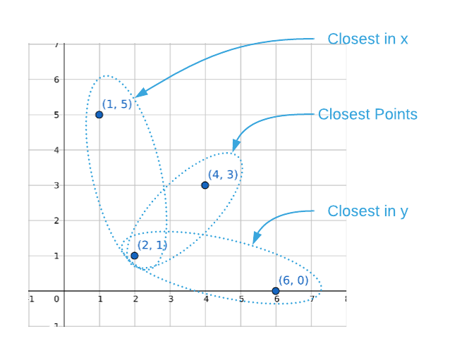
Recall that the final one-dimensional algorithm is $O(n \log_2{n})$. It may be surprising to find that’s also possible to achieve the same runtime with two dimensions using similar techniques. However, sorting the values and performing a linear scan isn’t an option because it’s only possible to sort on a single dimension at a time. As the image below illustrates, closeness on a single axis does not indicate closeness across both axes.
This is not meant to imply that sorting isn’t useful to the two-dimensional problem, rather it’s an integral part of the solution. Likewise, linear scanning is indispensable. However, the application of the techniques isn’t as straightforward. The algorithm is complex so it’s prudent to start at the beginning. For the reader’s convenience, the prose below references pseudo code line numbers that correlate code to concepts.
Assume you need to find the closest points on the plane depicted below.
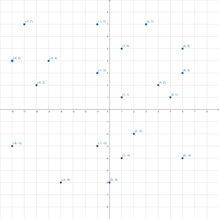
We begin almost identically to the one-dimensional divide and conquer algorithm.
Sort the data by the x coordinate (line 2), divide the points down the middle
(lines 15-17) and recursively calculate the closest distance (lines 34-35). See
the illustration below.
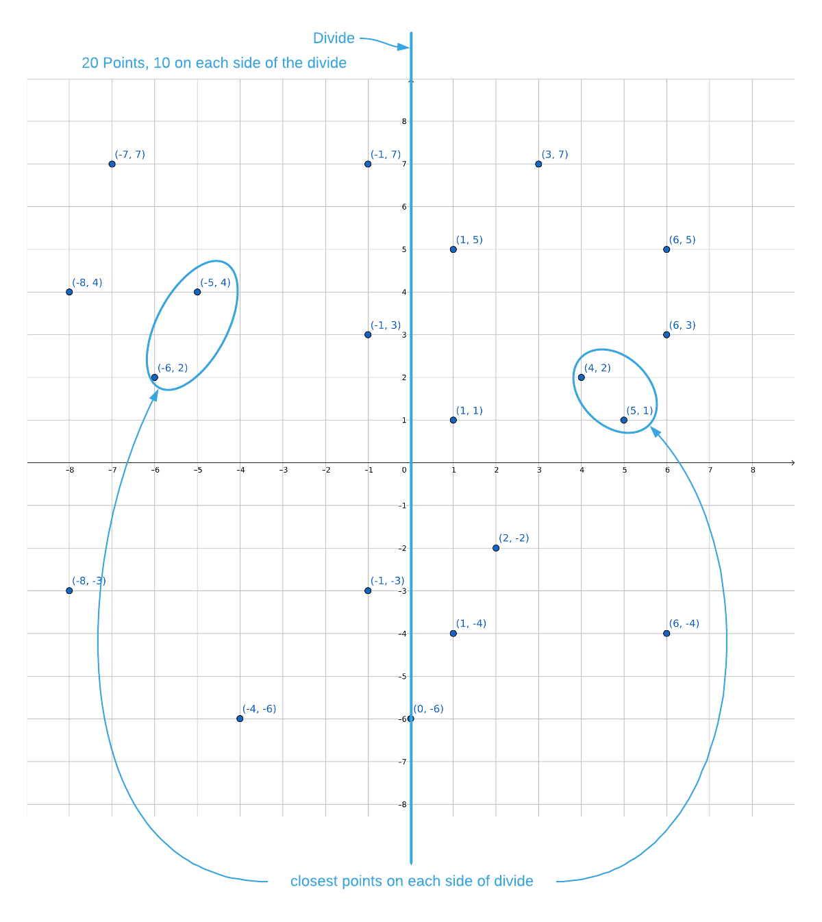
The closest pair in the left-side data cut is $(-5, 4), (-6, 2)$ and the closest pair in the right-side data cut is $(4, 2), (5, 1)$. The closest of the two is the latter, which makes the smallest known distance (line 37):
\[p1 = (4, 2)\\ p2 = (5, 1)\\ d(p1, p2) = \sqrt {(5 - 4)^2 + (1 - 2)^2} \approx 1.41\]At this point, there are two possible options for closest distance:
- The minimum of the left-side and the right-side recursive results, which is $\approx 1.41$.
- The distance between any one of the points on the left and any one of the points on the right: a split pair.
One option to find the closest split pair is to simply brute force compare all points on the left to all points on the right resulting in $\frac{n^2}{4}$ operations. However, recall that the goal is $O(n \log_2{n})$ overall. In order to achieve this runtime, finding the closest split pair must be strictly linear.
There is a way to quickly eliminate some of the points. It’s known that the closest distance on either side of the divide is 1.41; therefore, it stands to reason that both points in a split pair must be less than 1.41 from the divide (lines 40-46). This is best explained visually. See the graphic below.
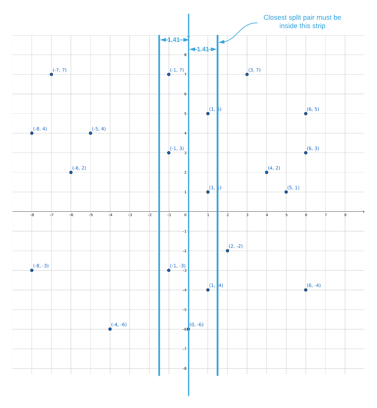
In the majority of cases, eliminating points outside the “strip” significantly
reduces the search space. It is however possible, in the worst case scenario,
that every point falls within the strip leaving the search space unchanged.
Luckily, the strip has some useful properties to exploit. Starting at the top of
the strip and moving down along the y axis, the only points that that need to
be considered are points where the y coordinates are less than 1.41 apart
(lines 49-59). See the image below.
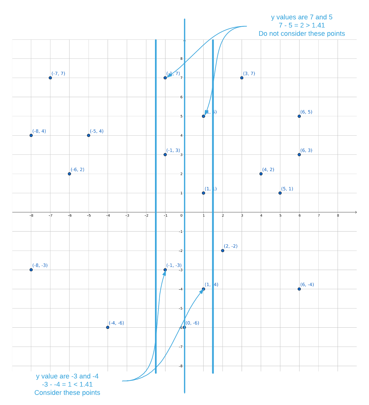
There is a proof5 that establishes the fact that each point within the strip will require no more than 6 comparisons (see the comment at line 51). This is truly remarkable so consider it carefully. Assume that the minimum distance found in the left and right side of the data is $\epsilon$. The proof states: within the strip, there cannot be more than 7 points within an $\epsilon$ sized span. What this means is that the maximum number of required comparison is $6n$; that is, 6 comparisons for every point in the strip. $6n$ is linear so the target runtime is achievable.
In a nutshell, finding the closest split pair is a matter of identifying the
points that lie within the “strip” (lines 40-46) and scanning them from top to
bottom (lines 49-59). A top to bottom scan requires sorting the data by the y
coordinate and up to this point the algorithm depends on the data being sorted
by the x coordinate. Resorting the points is an $O(n \log_2{n})$ operation.
That won’t do because in order to achieve the target runtime, finding the
smallest split pair must be linear. To avoid an extra sort operation, the
algorithm creates two copies of the points in a pre-processing step (line 3).
One copy is sorted by the x coordinate and the other by the y coordinate.
A problem arises because the recursive function (line 7) expects two copies of
the same points. The only difference between the two sets of points is the
sort order. Each recursion splits the data in half. Splitting the x-sorted
data is trivial (lines 15-17). However, the same cannot be said for the
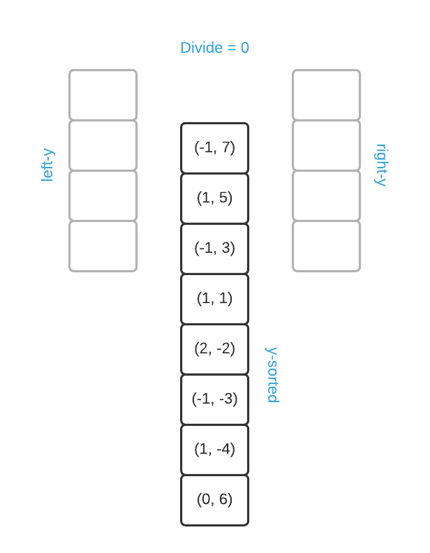
y-sorted points. The solution is to reverse merge6 the y-sorted
points into separate lists using the x coordinate as the dividing point (lines
24-32). The result is two lists with the same points as the x-sorted split
data while maintaining the y sort order. This image below depicts the process.
At this point, some confusion is to be expected. The algorithm has many moving parts and the description omits a few details for the sake of brevity. The following is a high-level summary intended to bring everything into focus.
To sum this up, the algorithm is defined as follows:
- Sort the data by the
xandycoordinate, we’ll call the resulting listsAxandAy(lines 2-3) - Divide
Axdown the middle creating two lists of size $\frac{n}{2}$, we’ll call themleft-cutandright-cut(lines 15-17) - Reverse merge
Ayinto two lists of size $\frac{n}{2}$, we’ll call the resulting listsleft-yandright-y- the same points asleft-cutandright-cutwith a different sort order (lines 24-32) - Recursively find the closest pair in
left-cutandright-cut, sendingleft-yandright-yalong for the ride (lines 34-35) - Find the minimum distance returned from the two recursive calls, we’ll call
this distance
closest-dist(line 37) - Find the closest split pair, that is, a pair where one point exists in
left-cutand one exists inright-cut- Create a
stripby eliminating all points fromAythat are more thanclosest-distfrom from the dividing point on thexaxis (lines 39-46) - Scan
stripfrom top to bottom only considering points whereyis less thanclosest-distfrom its predecessor. If the distance between any of the points is less thanclosest-dist, overwriteclosest-dist(lines 49-49)
- Create a
- Return
closest-dist(line 61)
Don’t worry if the details are still fuzzy. The average reader will need to reread this subsection several times before tackling the exercises. Like most things worth knowing, it takes work. As an added bonus, the concepts set forth here are easily transferable to three-dimensions.
Applications
- Robotics
- Computer Vision
- Graphics
- Airline traffic control
Pseudo Code
\begin{algorithm}
\caption{Closest Points}
\begin{algorithmic}
\REQUIRE A = set of 2-tuples representing x and y coordinates on a plane having $\vert A \vert \geq 2$
\OUTPUT the distance between the two closest points as measured by Euclidean distance
\FUNCTION{closestPair}{A}
    \STATE Ax $\gets$ A sorted by the x coordinate
    \STATE Ay $\gets$ A sorted by the y coordinate
    \RETURN \CALL{closestPairRecursive}{$Ax$, $Ay$}
\ENDFUNCTION
\STATE
\REQUIRE Ax = set of 2-tuples representing x and y coordinates sorted by the x corrdinate
\REQUIRE Ay = set of 2-tuples representing x and y coordinates sorted by the y corrdinate
\OUTPUT the distance between the two closest points as measured by Euclidean distance
\FUNCTION{closestPairRecursive}{Ax, Ay}
    \STATE $n \gets \vert Ax \vert$
    \STATE
    \IF{n $\leq$ 3}
        \RETURN \CALL{closestPairBruteForce}{Ax}
    \ENDIF
    \STATE
    \STATE \COMMENT{Divide the points down the middle of the x axis}
    \STATE mid $\gets \floor{\frac{n}{2}}$
    \STATE left-cut $\gets$ $\{Ax_0...Ax_{\text{mid} - 1}\}$
    \STATE right-cut $\gets$ $\{Ax_{\text{mid}}...Ax_{n-1}\}$
    \STATE
    \STATE \COMMENT{This x value is the dividing point}
    \STATE divide $\gets Ax_{\text{mid -1}}.x$
    \STATE
    \STATE \COMMENT{Split the y-sorted points into halves that match left-cut and right-cut}
    \STATE \COMMENT{This eliminates the need for an additonal $O(n \log_2{n})$ sort operation}
    \STATE left-y $\gets \emptyset$
    \STATE right-y $\gets \emptyset$
    \FOR{$i \in Ay$}
        \IF{$i.x \leq$ divide}
            \STATE left-y $\gets \text{left-y} \cup \{i\}$
        \ELSE
            \STATE right-y $\gets \text{right-y} \cup \{i\}$
        \ENDIF
    \ENDFOR
    \STATE
    \STATE left-closest-dist $\gets$ \CALL{closestPairRecursive}{left-cut, left-y}
    \STATE right-closest-dist $\gets$ \CALL{closestPairRecursive}{right-cut, right-y}
    \STATE
    \STATE closest-dist $\gets$ \CALL{min}{left-closest-dist, right-closest-dist}
    \STATE
    \STATE \COMMENT{Create the strip}
    \STATE strip $\gets \emptyset$
    \FOR{$i \in Ay$}
        \STATE \COMMENT{$\vert \vert$ denotes absolute value in this instance}
        \IF{$\vert i.x - \text{divide} \vert \lt$ closest-dist}
            \STATE strip $\gets \text{strip} \cup \{i\}$
        \ENDIF
    \ENDFOR
    \STATE
    \STATE \COMMENT{Compare each point in the strip to the points within closest-dist below it}
    \FOR{$i \gets 0$ to $\vert\text{strip}\vert$}
        \STATE $j \gets i + 1$
        \STATE \COMMENT{This while loop will never execute more than 6 times}
        \WHILE{$j < \vert\text{strip}\vert$ and $(\text{strip}_{j}.y - \text{strip}_i.y) \lt$ closest-dist}
            \STATE dist $\gets$ \CALL{distance}{$\text{strip}_i, \text{strip}_j$}
            \IF{dist $\lt$ closest-dist}
                \STATE closest-dist $\gets$ dist
            \ENDIF
            \STATE $j \gets j + 1$
        \ENDWHILE
    \ENDFOR
    \STATE
    \STATE return closest-dist
\ENDFUNCTION
\STATE
\REQUIRE $p1, p2$ = 2-tuples representing x and y coordinates
\OUTPUT Euclidean distance between p1 and p2
\FUNCTION{distance}{$p1$, $p2$}
    \RETURN $\sqrt{(p2_x - p1_x)^2 + (p2_y - p1_y)^2}$
\ENDFUNCTION
\end{algorithmic}
\end{algorithm}
Asymptotic Complexity
- Naive - $O(n^2)$
- Divide and Conquer - $O(n \log_{2} n)$
Actual Run Times
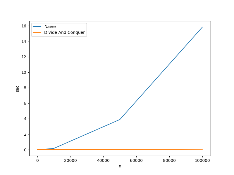
There is no doubt that the divide and conquer version of the closest pair algorithm is considerably more cognitively complex than the brute force version. Questioning its efficacy is perfectly justifiable. The cardinal rule of algorithm design is: when in doubt, collect empirical data. The chart and table below outline actual run times.
| Algorithm | n=100 | n=1000 | n=10000 | n=50000 | n=100000 |
|---|---|---|---|---|---|
| Naive | 0.000020 sec | 0.002366 sec | 0.156841 sec | 3.888813 sec | 15.825694 sec |
| Divide And Conquer | 0.000023 sec | 0.000353 sec | 0.003710 sec | 0.021901 sec | 0.045483 sec |
Key Takeaways:
- The divide and conquer algorithm is $\approx$ 350 times faster with an input of 100,000 points.
- Assuming that the use case calls for large data sets, the additional cognitive complexity is warranted.
Source Code
Relevant Files:
Click here for build and run instructions
Exercises
-
In the case of the one-dimensional closest pair algorithm, what is the advantage of the divide and conquer approach over the simple sorting and scanning approach.
Answers (click to expand)
There is no advantage. The sorting and searching approach is less cognitively complex and more performant. The only reason it's included in this material is that it provides a gentle introduction to concepts required for the two-dimensional problem.
-
Lines 15 thru 17 of the pseudo code divide the points down the middle of the
x-axis. Lines 40 thru 46 create an imaginary “strip” that spans the dividing point. How wide is this strip?Answers (click to expand)
Assuming the minimum distance found in the left and right cuts is $\epsilon$, the strip is $2\epsilon$ wide. It's not possible for a split pair to be closer together than $\epsilon$ and also be farther than $\epsilon$ from the dividing point.
-
Answer each of the following questions True or False:
a. Eliminating all points outside of the “strip” is guaranteed to reduce the search space.
b. Assuming the minimum distance found in the left and right cuts is $\epsilon$, it’s not possible for more than 7 points to reside within an $\epsilon$ sized span on theyaxis.Answers (click to expand)
- False - It's possible, in the worst case scenario, for all points to fall within the strip.
- True - This is a proven fact.
-
Using the programming language of your choice, implement the closest pair algorithm. The
closestPairfunction of the pseudo code returns just the closest distance; however, your implementation should also return the pair of points.Answers (click to expand)
See the C implementation provided in the links below. Your implementation may vary significantly and still be correct.
- closest_pair.h
- closest_pair.c
- closest_pair_test.c -
Lines 26 thru 32 of the pseudo code impose a non-obvious constraint on the input data. Describe the constraint.
Answers (click to expand)
The constraint is that all the
xvalues must be distinct. To demonstrate, suppose you have the following five points passed in at line 7: \(Ax \gets \{(2,7), (3, 2), (3,9), (3,6), (7,10)\} \\ Ay \gets \{(3, 2), (3,6), (2,7), (3,9), (7,10)\}\) That is, the same five points sorted first by thexcoordinate and then by theycoordinate. Notice that three of the points share the samexcoordinate. Lines 16 and 17 divide $Ax$ into two sets: \(\text{left-cut} \gets \{(2,7), (3, 2)\} \\ \text{right-cut} \gets \{(3,9), (3,6), (7,10)\}\) Thedividevariable is set to 3 on line 20. The purpose of lines 26 thru 31 is to createy-sorted versions ofleft-cutandright-cutand store them inleft-yandright-yrespectively. Because line 27 is only considering thexvalue, the result is: \(\text{left-y} \gets \{(3,2), (3, 6), (2, 7), (3, 9)\} \\ \text{right-y} \gets \{(7,10)\}\) At this point,left-cutandleft-ydo not contain the same points and the same is true ofright-cutandright-y. The algorithm will not return the correct answer. -
Modify the code you created for exercise 4 to remove the constraint identified in question 5. It is acceptable to assume your algorithm will not have to deal with duplicate points, that is, points were
xandyare both identical.Answers (click to expand)
See the C implementation provided in the links below. Your implementation may vary significantly and still be correct.
- closest_pair.h
- closest_pair.c
- closest_pair_test.c
See the pseudo code solution here. -
The points.txt file contains one million unique Cartesian coordinates. There are duplicate
xandyvalues, but each point is unique. Each coordinate is on a separate line and the format of each line is a follows:
{x},<space>{y}.
Find the closest pair contained in the file.Answers (click to expand)
See the
Cimplementation provided in theFindClosestPairInFilefunction located in this file: closest_pair_test_case.c. Your implementation may vary significantly and still be correct. The final output should be:
Point 1=(38524.043694, -33081.291468), Point 2=(38523.977990, -33081.309257), Distance=0.068070.
For reference, theCimplementation completed the task in $\approx$ 900 milliseconds running on a Surface Book 2 Laptop (Intel Core i7, 16 GB RAM).
-
Available online at https://ieeexplore.ieee.org/document/4567872 ↩
-
Consult the Graphing prerequisite if you need a more in-depth concept review. ↩
-
Typically represented by a 2-tuple in the form of
(x, y)↩ -
For the sake of accuracy, Cartesian coordinates can also be used to specify points on a three-dimensional plane. ↩
-
See section 33.4 on page 1039 of Introduction to Algorithms, 3rd Edition by Thomas H. Cormen, Charles E. Leiserson, Ronald L. Rivest, and Clifford Stein. ↩
-
Essentially, a reverse merge is the opposite of merge sort’s combine step. Merge sort combines two lists into one and reverse merge splits a single list into two smaller lists. ↩