Priority Queue

graph LR
	ALG(["fas:fa-trophy Priority Queue fas:fa-trophy #160;"])

	ASY_ANA(["fas:fa-check Asymptotic Analysis #160;"])
    click ASY_ANA "./math-asymptotic-analysis"

	ARRAY(["fas:fa-check Array #160;"])
    click ARRAY "./list-data-struct-array"

	BT(["fas:fa-check Binary Tree #160;"])
    click BT "./list-data-struct-binary-tree"

	QUEUE(["fas:fa-check Queue #160;"])
    click QUEUE "./data-struct-queue"

	ASY_ANA-->ALG
    ARRAY-->ALG
    BT-->ALG
    QUEUE-->ALG

The Queue data structure is well suited to tracking linear lists. That is, lists whose elements can only be accessed in sequential order (First-In-First-Out). Unfortunately, not all lists are linear in nature. Priority based retrieval of items (priority-in-first-out)¹ is a common requirement. For instance, a logical queue is useful for letting people into a night club. The person standing in line the longest should be let in first. However, emergency room admittance is based on a priority. If a person with a potentially fatal injury arrives after a person with a stubbed toe, that person has priority and should be admitted first. This scenario calls for a priority queue that will always return the highest priority items first regardless of the insertion order.

History

In 1954, Alan Cobham introduced the concept of a priority queue in his paper entitled Priority Assignment in Waiting Line Problems². This was a seminal work for queuing theory and it had a notable impact on the computing industry. Priority queues became a software staple in 1964 when John William Joseph Williams published the Heap Sort Algorithm in the ACM Journal³. Unfortunately, the quick sort algorithm, discovered by Tony Hoare in 1959 generally outperforms it. In spite of its relative failure, the heap data structure is perfectly suited as a priority queue implementation. In fact, it is so useful that the terms heap and priority queue are often used interchangeably.

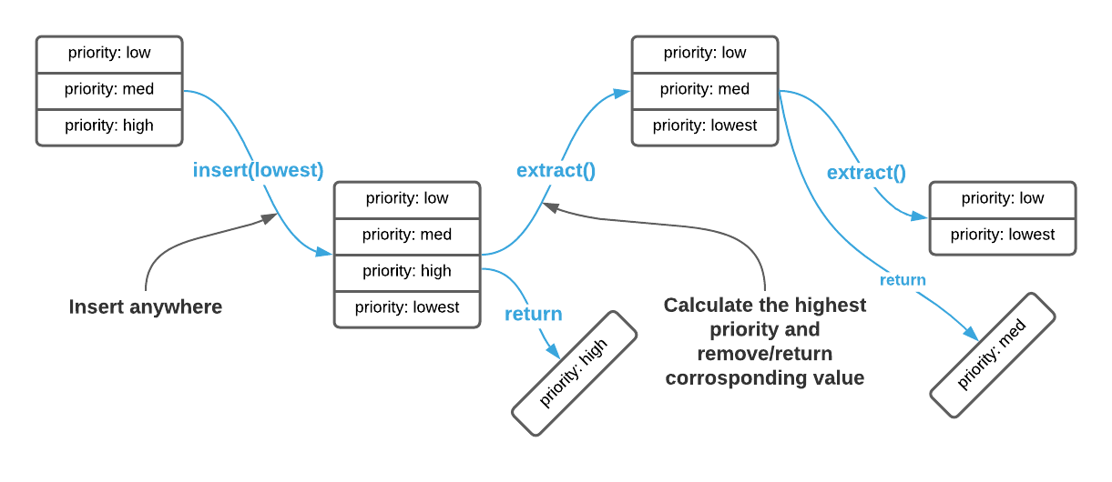
The abstract interface of a priority queue has two operations: insert and extract⁴. See the supplied Pseudo Code. insert adds an element to the priority queue. extract returns the element with the highest priority. This is illustrated in the image below.

A key concept here is priority. It’s often difficult to grasp because the definition is application dependent. In some cases items are prioritized based on the ordinal position of an integer key, others may rank priority by largest number, others may rank on a combination of data attributes. In this sense, no two priority queues are alike. Most implementations allow the consumer to specify a priority function that determines the relative importance of nodes.

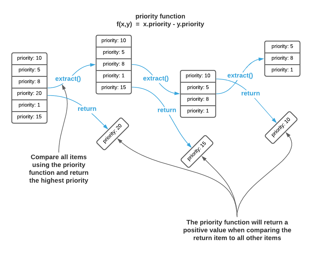
f(x, y) Priority Function

A priority function is a piece of code that compares two data elements and returns their relative priority, typically as an integer⁵. If the return value is negative the first element precedes the second, if it’s positive the first element succeeds the second, and if it’s zero the elements have equal priority. It’s possible to write a priority function to accommodate almost any prioritization scheme.

Consider a priority function that compares two integers, if the goal is to make the highest number the highest priority, the function is defined as follows:

Now consider a priority function that ranks lower numbers with higher priority.

The concept is shown graphically below.

The graphic above depicts the logical operation of a priority queue. The purpose is to present an easy to understand description of the abstract interface. It provides enough information to efficiently consume a pre-made priority queue. However, an exact implementation as shown above results in a $\Theta(n^2)$ algorithm because extract requires comparison of every element to every other element. The innovation behind priority queue implementations is reducing the total number of comparisons. Before moving on, try to conceive of a few of your own.

There are many efficient priority queue implementations, the most popular of which is a heap⁶.

Heap

A heap arranges data in such a way that the highest priority element is always retrievable in constant ($\Theta(1)$) time. They are logically similar to Binary Trees but are stored in memory as Arrays. First, consider the logical layout of a heap as a tree.

A heap is a tree that maintains the following invariants⁷:

1. The highest priority node resides at the root
2. Every node has as most 2 children
3. Every layer of the tree is as full as possible
4. Every node has an equal or higher priority than it’s children

This concept is best understood visually. See the image below. Assume that the priority function ranks lower numbers highest ($f(x, y) = y - x$).

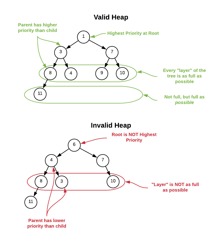
The invariants are somewhat lax. There are many valid ways to organize data while maintaining these properties. The key thing to note is that the highest priority element is always located at the root making it easily accessible. Additionally, the data is not optimized for searching. The only guarantee is that all child nodes have lower priority than their upward ancestry. There is no indication of which path (left or right) a particular value exists in. Therefore, locating specific values in the tree is an $O(n)$ operation. The heap logical structure is solely optimized for locating high priority elements.

The image above is logically sound; however, it’s a bit misleading from a memory layout perspective. Unlike binary trees, the arrows do not represent pointers, rather they represent relationships. A heap stores all nodes in an array and locates it’s ancestry via simple index calculations. The root node is always located at index 0 and the formulas below describe how to locate each logical node in the array. Assume i is the index of the node in question.

• Parent Node Index = $\left \lfloor \frac{i + 1}{2} \right \rfloor - 1$
• Left Child Index = $2(i + 1) - 1$
• Right Child Index = $2(i + 1)$

This is a difficult concept to understand without a visual. Please see the image below.

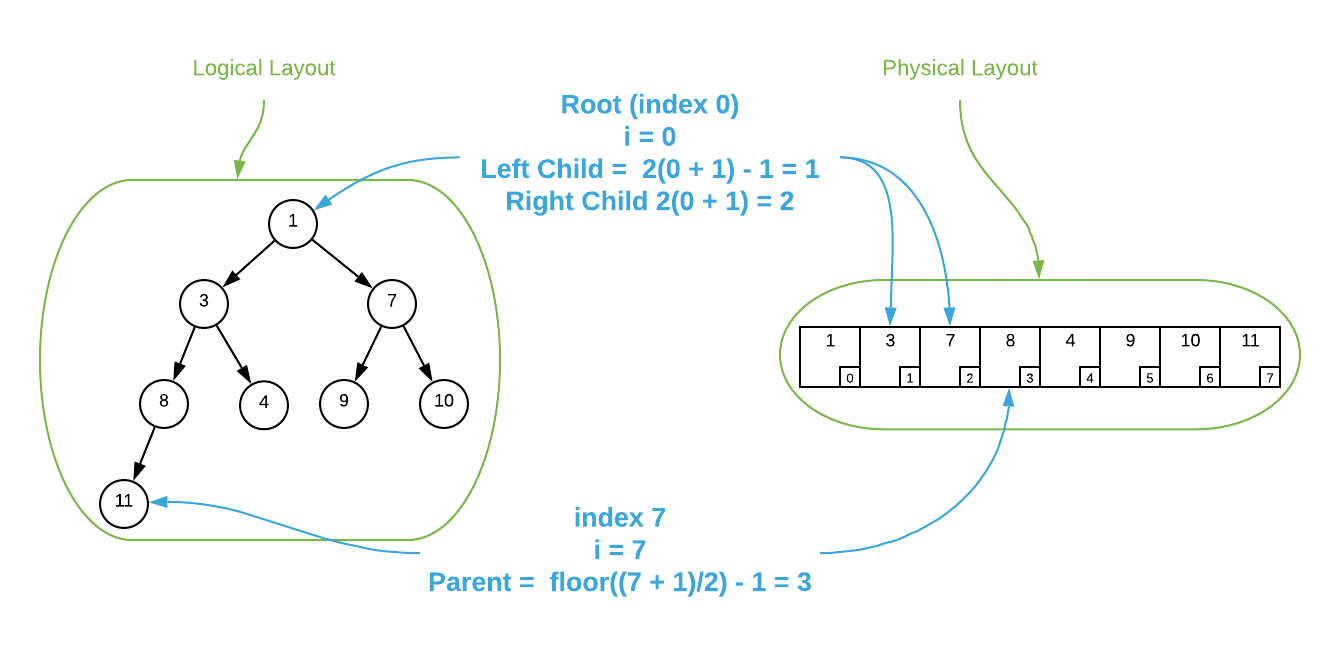
To further illustrate the concept, consider the item located at index $\blue{3}$ in the array depicted above. It holds the value of 8. The calculation to locate its parent is $\left \lfloor \frac{\blue{3} + 1}{2} \right \rfloor - 1 = 1$. The value stored at index 1 is 3. As you can see, it is the parent node. To locate the left child, the calculation is $2(\blue{3} + 1) - 1 = 7$. The value 11 is stored at index 7 and it is indeed the left child. Calculating the right child results in a number that’s outside the bounds of the array.

Do not be alarmed if this seems a bit abstruse. The concept takes some getting used to. If you’re struggling, study the pseudo code below and re-read this section.

Heap Pseudo Code

\begin{algorithm}
\caption{Heap}
\begin{algorithmic}
\REQUIRE func = priority function
\REQUIRE size = maximum number of elements the heap can store
\OUTPUT heap data structure
\FUNCTION{create}{func, size}
    \STATE heap $\gets$ new memory allocation
    \STATE heap.priorityFunc $\gets$ func
    \STATE heap.data $\gets$ array of size
    \STATE heap.maxSize $\gets$ size
    \STATE heap.itemCount $\gets$ 0
    \RETURN{heap}
\ENDFUNCTION
\STATE
\REQUIRE heap = heap data structure
\REQUIRE value = value to add to the heap
\FUNCTION{insert}{heap, value}
    \IF{heap.itemCount = heap.maxSize}
        \STATE overflow
    \ENDIF
    \STATE heap.data[heap.itemCount] $\gets$ value
    \STATE bubbleUpIndex $\gets$ heap.itemCount
    \STATE heap.itemCount $\gets$ heap.itemCount + 1
    \STATE \CALL{bubbbleUp}{heap, bubbleUpIndex} \COMMENT{function defined below}
\ENDFUNCTION
\STATE
\REQUIRE heap = heap data structure
\OUTPUT value with the highest priority
\FUNCTION{extract}{heap}
    \IF{heap.itemCount = 0}
        \STATE underflow
    \ENDIF
    \STATE returnValue $\gets$ heap.data[0]
    \STATE heap.itemCount $\gets$ heap.itemCount - 1
    \STATE heap.data[0] $\gets$ heap.data[heap.itemCount]
    \STATE bubbleDownIndex $\gets$ 0
    \STATE \CALL{bubbbleDown}{heap, bubbleDownIndex} \COMMENT{function defined below}
    \RETURN{returnValue}
\ENDFUNCTION
\STATE
\REQUIRE i = index of the item to find the parent for
\OUTPUT index of parent item
\FUNCTION{parentIndex}{i}
    \RETURN{$\left \lfloor \frac{i + 1}{2} \right \rfloor - 1$}
\ENDFUNCTION
\STATE
\REQUIRE i = index of the item to find the left child for
\OUTPUT index of left child item
\FUNCTION{leftChildIndex}{i}
    \RETURN{$2(i + 1) - 1$}
\ENDFUNCTION
\STATE
\REQUIRE i = index of the item to find the right child for
\OUTPUT index of right child item
\FUNCTION{rightChildIndex}{i}
    \RETURN{$2(i + 1)$}
\ENDFUNCTION
\STATE
\REQUIRE heap = heap data structure
\REQUIRE index = index of the node to bubble up to it's correct location
\FUNCTION{bubbleUp}{heap, index}
    \WHILE{index $\neq$ 0}
        \STATE parentIndex $\gets$ \CALL{parentIndex}{index}
        \IF{\CALL{heap.priorityFunc}{heap.data[index], heap.data[parentIndex]} $\leq$ 0}
            \RETURN{}
        \ENDIF
        \STATE swap heap.data[index] and heap.data[parentIndex]
        \STATE index $\gets$ parentIndex
    \ENDWHILE
\ENDFUNCTION
\STATE
\STATE
\REQUIRE heap = heap data structure
\REQUIRE index = index of the node to bubble down to it's correct location
\FUNCTION{bubbleDown}{heap, index}
    \WHILE{\CALL{rightChildIndex}{index} $\lt$ heap.itemCount - 1}
        \STATE left $\gets$ \CALL{leftChildIndex}{index}
        \STATE right $\gets$ \CALL{rightChildIndex}{index}
        \IF{\CALL{heap.priorityFunc}{heap.data[left], heap.data[right]} $\geq$ 1}
            \STATE childIndex $\gets$ left
        \ELSE
            \STATE childIndex $\gets$ right
        \ENDIF
        \IF{\CALL{heap.priorityFunc}{heap.data[index], heap.data[childIndex]} $\geq$ 0}
            \RETURN{}
        \ENDIF
        \STATE swap heap.data[index] and heap.data[childIndex]
        \STATE index $\gets$ childIndex
    \ENDWHILE
\ENDFUNCTION
\end{algorithmic}
\end{algorithm}

As a final matter of note, there are many different heap variations. Presented above is a Binary Heap which is one of the simplest. Other types of heaps vary in run times and internal details, but they all operate similarly. An in-depth exploration of heap implementations falls outside of scope. It would be easy to write an entire book on the subject. To demonstrate the breadth of the topic, below is an incomplete list of heap variants.

• 2-3 heap
• B-heap
• Beap
• Binomial heap
• Brodal queue
• d-ary heap
• Fibonacci heap
• Leaf heap
• Leftist heap
• Pairing heap
• Radix heap
• Randomized meldable heap
• Skew heap
• Soft heap
• Ternary heap
• Treap
• Weak heap

Binary heaps are suitable for most general purpose applications. In the event that the reader has a need to implement a heap for a mission critical application, it’s highly recommended they research the topic more thoroughly. There are many heap variants that may or may not be better suited to specialized scenarios.

Applications

• Running Median
• Dijkstra’s Shortest Path
• Prim’s Minimum Spanning Tree
• Huffman Codes
• Load balancing
• Interrupt handling
• Any algorithm requiring repeated min/max lookups

Pseudo Code

\begin{algorithm}
\caption{Priority Queue Abstract Interface}
\begin{algorithmic}
\REQUIRE value = value to add to the queue
\FUNCTION{insert}{value}
    \STATE Q $\gets$ Q $\cup$ value
\ENDFUNCTION
\OUTPUT value with the highest priority
\FUNCTION{extract}{}
    \STATE value $\gets$ value having $\max({\text{priority} \in Q})$
    \STATE Q $\gets$ Q - value
    \RETURN{value}
\ENDFUNCTION
\end{algorithmic}
\end{algorithm}

Asymptotic Complexity

• Insert: $O(\log n)$
• Extract: $O(\log n)$

Source Code

Full Repo

Relevant Files:

• heap.h
• heap.c
• heap_test.c

Click here for build and run instructions

Exercises

1. Assuming the only options are stack, queue, and priority queue, choose the data structure most suited for each of the following applications.
   a. Tracking incoming customer support requests
   b. Buffering streaming video content
   c. Tracking incoming threats
   d. Backtracking (tracking user operations to enable undo functionality)

   Answers (click to expand)

   a. Queue, assuming all customers have equal priority.
   b. Queue, content should be displayed in the order it is received⁸.
   c. Priority Queue, higher priority threats should receive the most immediate attention.
   d. Stack, undo should reverse the last user operation.

2. Assume you have a pre-made priority queue that you are using to track inventory items. Each node in the priority queue has an associated cost and quantity. Specify a priority function that will rank items by:
   a. Highest Quantity
   b. Lowest Quantity
   c. Highest Total Cost ($\text{cost} \times \text{quantity}$)

   Answers (click to expand)

   1. $f(x, y) = x.\text{quantity}-y.\text{quantity}$
   2. $f(x, y) = y.\text{quantity}-x.\text{quantity}$
   3. $ f(x,y)=\begin {cases} \text{if} \quad (x.\text{quantity} \times x.\text{cost} \gt y.\text{quantity} \times y.\text{cost}) \quad \text{return } 1\\ \text{if} \quad (x.\text{quantity} \times x.\text{cost} \lt y.\text{quantity} \times y.\text{cost}) \quad \text{return} -1\\ \text{return } 0\ \end {cases} $
      Notice that simply returning $(x.\text{quantity} \times x.\text{cost}) - (y.\text{quantity} \times y.\text{cost})$ wont work. That pattern is only sufficient for integer values. To illustrate this, consider the case where $x = 0.75$ and $y = 0.5$. Clearly, $x$ should be prioritized before $y$ because $0.75 - 0.5 = 0.25$ and $0.25$ is $\gt 0$. However, converting $0.25$ to an integer return values yields $0$ which indicates equality.

3. The image below represents the memory layout of an integer heap that specifies the lowest value as the highest priority ($f(x, y) = x - y$). Assuming the logic specified in the heap pseudo code, answer the following questions.
   a. What, if any of the invariants are violated by this layout.
   b. Assume you execute BubbleUp(heap, 8). Draw the array as it would exist at each invocation of line 45.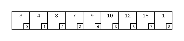

   

   Answers (click to expand)

   a. Invariants 1 and 4 are violated. Index 8, which has a value of 1 should be located at the root (index 0). Also, index 8 has a higher priority than it’s parent at index 3.
   b.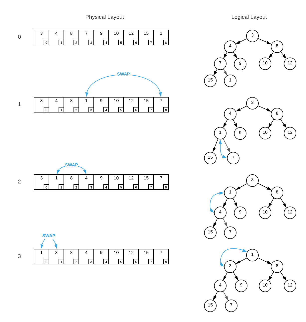

4. A common priority queue requirement is reprioritization. That is, updating the priority of an existing element. Augment the supplied heap pseudo code to add this functionality. Assume a consumer has the ability to manually change the priority data associated with an existing node in the heap. Define a function that accepts the index of a modified node and relocates it in the heap to maintain the invariants.

   For formatting purposes, the answers to question 4 are located here.

5. Using the programming language of your choice, implement a heap. Make the implementation detailed enough for you to fully grasp the intricacies of the data structure.

6. Answer me these questions three:
   a. What is your name?
   b. What is your quest?
   c. What… is the air-speed velocity of an unladen swallow?

   Answers (click to expand)

   1. It is Arthur, King of the Britons
   2. To seek the Holy Grail
   3. What do you mean? An African or European swallow?