Prerequisites (click to view)
graph LR
	ALG(["fas:fa-trophy Merge Sort fas:fa-trophy #160;"])

	ASY_ANA(["fas:fa-check Asymptotic Analysis #160;"])
    click ASY_ANA "./math-asymptotic-analysis"

	ARRAY(["fas:fa-check Array #160;"])
    click ARRAY "./list-data-struct-array"

	ASY_ANA-->ALG
	ARRAY-->ALG
Merge sort is possibly the most popular sorting algorithm in use today. It is embedded in many popular languages such as Python, Java1, and Perl. While it’s considerably more complex than the previously covered algorithms, it’s runtime, both theoretically and in practice, is significantly better.
History
The EDVAC (Electronic Discrete Variable Automatic Computer) was the world’s first stored program computer. John Von Neumann published a paper in 1945 entitled First Draft of a Report on the EDVAC2, which described the machine’s physical architecture. Modern day computers still follow the same basic design, which has came to be known as Von Neumann Architecture. The first algorithm ever written for the EDVAC was merge sort.
Merge sort is asymptotically optimal meaning that it is mathematically provable3 that it is NOT possible to create a comparison-based sort algorithm that is faster by more than a constant factor. The hard limit for the worst-case4 runtime of any comparison-based sorting algorithm is $O(n \log_2{n})$. Merge sort is $\Theta(n \log_2 n)$ and is therefore asymptotically optimal. The implication is that while it is possible to improve on the best-case runtime ($\Omega$), it is not possible to improve on the worst-case asymptotic runtime ($O$).
Merge sort minimizes operations in a clever way. It splits the data in half, recursively sorts each half, and finally merges them together. Take a few moments to familiarize yourself with the algorithm by studying the pseudo code in conjunction with the image below. For an additional challenge, try to correlate lines of pseudo code with each outlined box.
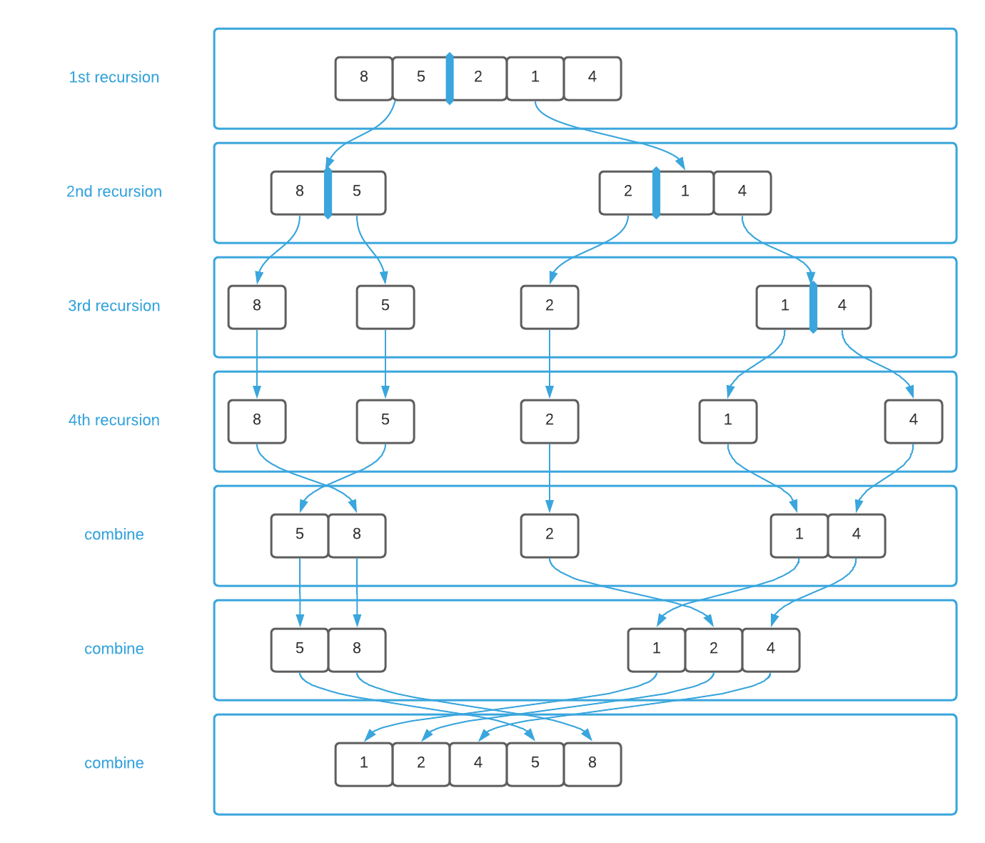
The basic design of merge sort is applicable in many other contexts. In fact, it’s common enough to have a name: divide and conquer.
Divide and Conquer
Merge sort is an example of the divide and conquer5 algorithm design paradigm. All algorithms of this ilk follow the same basic recipe.
- Divide the input into smaller sub problems
- Conquer the sub problems recursively
- Combine the solutions of the sub problems into a final solution
In the case of merge sort, step one is dividing the data in half, as shown in lines 6 thru 12 of the pseudo code. Lines 11 and 12 account for step two of the recipe. The algorithm continues to recurse until the data is separated down to its base case, which is defined on lines 2 thru 4. At this point, each individual data element is considered in isolation.
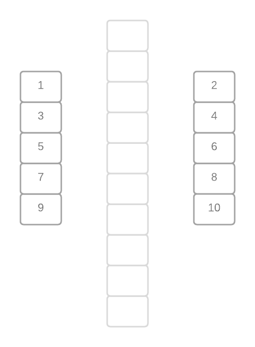
The third step of the recipe is always the most difficult. The merge sort combine step is defined in lines 17 thru 33 where the data is combined in sorted order. It’s helpful to envision this step like a zipper where each element is a tooth as illustrated graphically below.
This technique is a useful tool for your algorithm toolbox as the recipe generalizes to many problems.
Pseudo Code
\begin{algorithm}
\caption{Merge Sort}
\begin{algorithmic}
\REQUIRE $A$ = list of numbers
\OUTPUT Copy of $A$ sorted in sequential order
\FUNCTION{mergeSort}{$A$}
    \IF{$\vert A \vert = 1$}
        \RETURN A
     \ENDIF
     \STATE
     \STATE n $\gets \vert A \vert$
     \STATE half $\gets \floor{\frac{n}{2}}$
     \STATE A1 $\gets \{A_0...A_{\text{half}}\}$
     \STATE A2 $\gets \{A_{\text{half} + 1}...A_{n - 1}\}$
     \STATE
     \STATE A1 $\gets$ \CALL{mergeSort}{A1}
     \STATE A2 $\gets$ \CALL{mergeSort}{A2}
     \STATE
     \STATE B $\gets$ empty array
     \STATE A1-position $\gets$ 0
     \STATE A2-position $\gets$ 0
     \FOR{i $\gets$ 0 to n}
        \IF{A1-position $\geq \vert A1 \vert$}
            \STATE $\{B_i...B_{n - 1}\} \gets \{A2_{\text{A2-position}}...A2_{\vert A2 \vert - 1}\}$
            \BREAK
        \ELSEIF{A2-position $\geq \vert A2 \vert$}
            \STATE $\{B_i...B_{n - 1}\} \gets \{A1_{\text{A1-position}}...A1_{\vert A1 \vert - 1}\}$
            \BREAK
        \ELSE
            \IF{$A1_{\text{A1-position}} \lt A2_{\text{A2-position}}$}
                \STATE $B_i \gets A1_{A1-position}$
                \STATE A1-position $\gets$ A1-position + 1
            \ELSE
                \STATE $B_i \gets A2_{A2-position}$
                \STATE A2-position $\gets$ A2-position + 1
            \ENDIF
        \ENDIF
     \ENDFOR
     \STATE
     \RETURN{B}
\ENDFUNCTION
\end{algorithmic}
\end{algorithm}
Asymptotic Complexity
$\Theta(n \lg_{2}n)$
Source Code
Relevant Files:
Click here for build and run instructions
Exercises
-
Compare the asymptotic memory consumption of the selection and merge sort algorithms.
Answers (click to expand)
Selection sort consumes a constant ($\Theta(1)$) amount of memory, meaning that it will use the same amount of memory regardless of the input size (see line 3 of the selection sort pseudo code). Conversely, merge sort consumes memory linear ($\Theta(n)$) to the size of the input (see line 14 of the merge sort pseudo code). Stated differently, the selection sort algorithm sorts data in place while merge sort transfers the data to an entirely new memory location leaving the original data untouched. As a final consideration, selection sort is not recursive while merge sort is; therefore, in the absence of a tail-call optimized language, merge sort consumes more stack space.
-
Answer each of the following questions True or False:
a. It is impossible to create an algorithm that performs better than merge sort.
b. Merge sort will always outperform bubble sortAnswers (click to expand)
- False: It is possible to create a more performant comparison-based sorting algorithm by reducing the number of operations. However, it's impossible to reduce the number of operations by more than a constant factor. Additionally, as demonstrated previously, it's possible to create an algorithm with a superior best case runtime.
- False: Bubble sort has a $\Omega(n)$ runtime. When the data is pre-sorted, it will outperform merge sort.
-
Using the programming language of your choice, implement a merge sort function that accepts:
- an array of any type
- a sorting strategy
Answers (click to expand)
See the C implementation provided in the links below. Your implementation may vary significantly and still be correct.
-
Instrument your merge sort algorithm to calculate the total number of copy and comparison operations. Next, sort the data contained in the sort.txt file and determine the total number of copy and comparison operations.
Answers (click to expand)
See the C implementation provided in sort_implementation.c Your implementation may vary significantly and still be correct. The final output should be:
Merge Sort: copy = 133,616 comparisons = 120,473 total = 254,089Comparing this to the number of operations preformed by the previous algorithms reveals why merge sort is faster in practice.
      Bubble Sort: copy = 71,844,390 comparisons = 49,988,559 total = 121,832,949
    Insertion Sort: copy = 23,968,128 comparisons = 23,958,117 total =  47,926,245
    Selection Sort: copy =     29,964 comparisons = 49,995,000 total =  50,024,964
        Merge Sort: copy =    133,616 comparisons =    120,473 total =     254,089
-
To satisfy my pedantic readers, Python and Java use Timsort, which incorporates merge sort into the overall algorithm. ↩
-
Available online at http://web.mit.edu/STS.035/www/PDFs/edvac.pdf ↩
-
See Chapter 8 of Introduction to Algorithms, 3rd Edition by Thomas H. Cormen, Charles E. Leiserson, Ronald L. Rivest, and Clifford Stein ↩
-
Some algorithms, such as bubble and insertion sort capitalize on portions of the data that are pre-sorted to achieve fewer operations. However, the said hard limit pertains to the worst case scenario. ↩
-
The phrase divide and conquer – divide et impera in Latin – originates with Julius Cesar. It denotes the military strategy he used to defeat the Gauls. ↩