Array

graph LR
	ALG(["fas:fa-trophy Array fas:fa-trophy #160;"])

	ASY_ANA(["fas:fa-check Asymptotic Analysis #160;"])
    click ASY_ANA "./math-asymptotic-analysis"

	ASY_ANA-->ALG

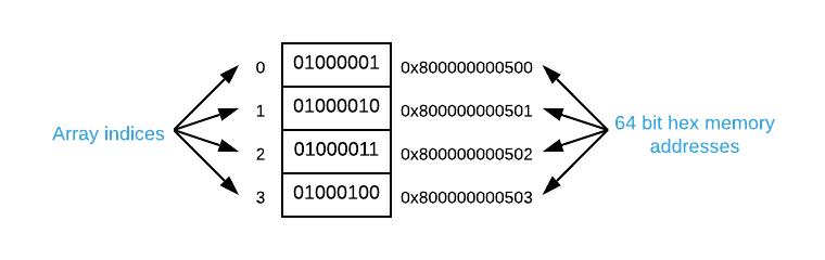
The array is the most common list data structure. Essentially, it’s nothing more than a contiguous section of memory filled with uniformly sized items stacked directly next to one another. The index of an item indicates its ordinal position in the array. Unlike many other data structures, arrays do not store any data above and beyond their constituent items. The image below depicts the memory layout¹ of an array containing the four ASCII² characters A, B, C, and D.

History

The array data structure dates back to the earliest digital computers. The first high-level programming language, Plankalkül, had an array data type. It was written by Konrad Zuse between 1942 and 1945. This is likely the origin of the concept as conceived today.

One could easily make the argument that arrays pre-date Plankalkül because they are often employed conceptually in assembly language³. For instance, John von Neumann created the merge sort algorithm using assembly in 1945 to sort array items. However, assembly language does not have an explicit array data type.

Size

Every array item must be the same size as measured in bytes (the reasons for this will be made clear in Direct Addressing). An item may span multiple bytes but cannot occupy a partial byte. ASCII characters have a size of 1 because they span a single byte. As another example, a 16-bit (2 bytes) integer has a size of 2. The graphic below illustrates the layout of an array containing the four 16-bit integers 1, 2, 3, and 4.

Direct Addressing

A distinct advantage of arrays is direct addressing⁴. The address of any item is easily calculable given the base address and index. Most high-level programming languages have an array abstraction that locates items using bracket syntax (something similar to array[index]). Behind the scenes, the program calculates the item’s address using a simple formula which is outlined below. Assume $i$ represents the desired index, $s$ represents the item size, and $a$ represented the base address.

For example, the graphic below outlines how to apply the formula to calculate the direct address of item 1 in an integer array.

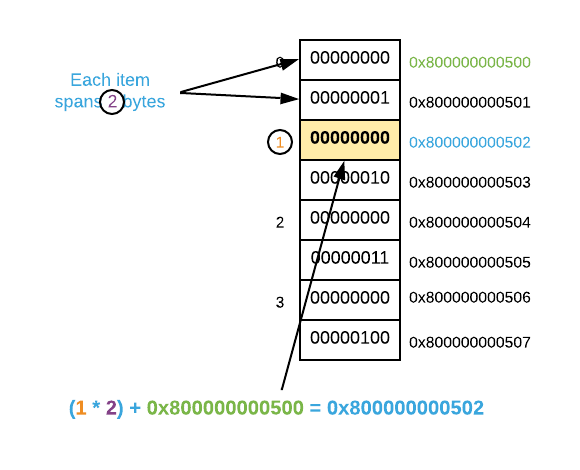
The consequence of direct addressing is that item retrieval is a constant ($O(1)$) operation. A common question amongst inquisitive programmers is, “why are array indices zero based?”. The simple answer⁵ is that it makes for easy math. Using the formula outlined above, the first item (index 0) in an array is \(0 * s + a\) which will always result in the base address.

Multi-Dimensional Arrays

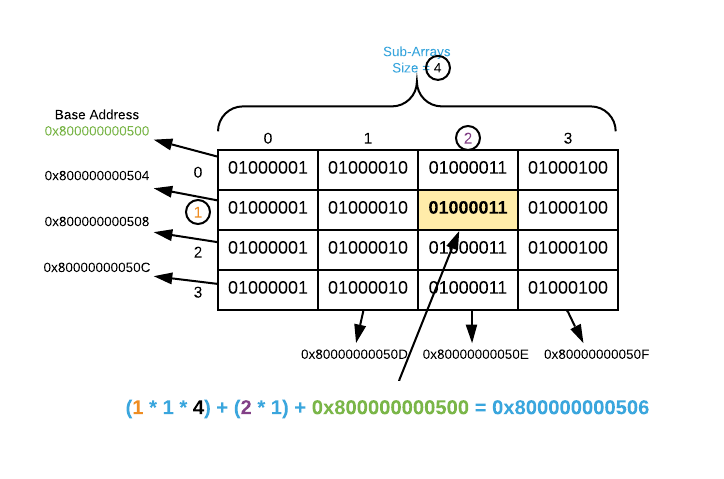
It’s easy to extend arrays to multi-dimensional arrays⁶. The only difference between an array and a multi-dimensional array is the direct address formula which is shown below. $i_1$ represents the index of the first array, $i_2$ represents the index of the sub array, $s$ represents the item size, $d$ represents the number of items in each sub array, and $a$ represents the base address.

This can be a bit confusing without a concrete example. Consider the multi-dimensional array of ASCII characters portrayed below. The image illustrates how to locate the address of item [1][2].

It’s theoretically possible to represent any number of dimensions by further extending the direct address formula. However, it’s rare to encounter more than 3-dimensions in the real world⁷. A good exercise for highly ambitious readers is to define the direct address formula for a 3-dimensional array⁸.

Spatial Locality

Arrays have optimal spatial locality. The concept of locality is deeply steeped in computer architecture and a thorough treatment is out of scope⁹. The “readers digest version” is that machines are able to use cache hierarchies optimally when accessing neighboring data. In other words, repeatedly accessing adjacent memory locations is faster than repeatedly accessing separated memory locations.

This is best demonstrated with an example. Consider the following two loops, do you expect any difference in execution time?

  // Row order access
  for (size_t i = 0; i < n; i++) {
    for (size_t j = 0; j < n; j++) array[i][j]++;
  }

  // Column order access
  for (size_t i = 0; i < n; i++) {
    for (size_t j = 0; j < n; j++) array[j][i]++; // i and j are reversed
  }

Using an Intel Core i7-8650U with 16 GB RAM the first loop (row order access) is actually almost six times faster¹⁰ than the second (column order access). For a value of n = 10,000 the first loops executes in $\approx$0.278 seconds and the seconds takes $\approx$1.590 seconds. Most programmers have a hard time accepting this; therefore, the source code contains an example located in the locality directory. Execute the compare_times.sh script to run the experiment locally.

In conclusion, recall that an array is a contiguous section of memory which equates to optimal spatial locality. Although the time differential is often negligible, it’s a salient concern for performance critical applications. The actual run times presented at the end of this section highlight more examples.

Applications

• Countless general purpose programming tasks
• Building block for several primitive data types including string, matrix, and mathematical vector to name a few.
• Building block for several more complex data structures including heap, hash table, and bloom filter to name a few.

Pseudo Code

\begin{algorithm}
\caption{Array Operations}
\begin{algorithmic}
\REQUIRE A = array
\REQUIRE item = item to insert into the array
\OUTPUT $A \cup$ item
\FUNCTION{insert}{A, item}
    \STATE $A^{\prime} \gets$ memory allocation of size $\vert A \vert + 1$
    \FOR{$i \in A$}
        \STATE copy $i$ to $A^{\prime}$
    \ENDFOR
    \STATE copy item to $A^{\prime}$
    \RETURN $A^{\prime}$
\ENDFUNCTION
\STATE
\REQUIRE A = array
\REQUIRE item = item to delete from the array
\OUTPUT $A - item$
\FUNCTION{delete}{A, item}
    \STATE $A^{\prime} \gets$ memory allocation of size $\vert A \vert - 1$
    \FOR{$i \in A$}
        \IF{$i \neq$ item}
            \STATE copy $i$ to $A^{\prime}$
        \ENDIF
    \ENDFOR
    \RETURN $A^{\prime}$
\ENDFUNCTION
\STATE
\REQUIRE A = array
\REQUIRE item = item to search for
\OUTPUT item if it exists, otherwise NULL
\FUNCTION{search}{A, item}
    \FOR{$i \in A$}
        \IF{$i =$ item}
            \RETURN item
        \ENDIF
    \ENDFOR
    \RETURN NULL
\ENDFUNCTION
\STATE
\REQUIRE A = array
\REQUIRE func = function to apply to each item
\FUNCTION{enumerate}{A, func}
    \FOR{$i \in A$}
        \STATE \CALL{func}{item}
    \ENDFOR
\ENDFUNCTION
\end{algorithmic}
\end{algorithm}

Implementation Details

The insert and delete pseudo code can be a bit misleading. It not at all advisable to actually copy items one at a time to a new memory location. These operations are indeed $O(n)$, however, with the right code they are also $\Omega(1)$. Consider the following:

• Many languages have dynamic arrays which allocate additional empty space to accommodate insertions.
• The C library command realloc may be able to resize an array without copying memory from one place to another. If there is free space available at the end of the end of the array, it simply expands the allocation. It’s always feasible to shirk an allocation.
• In the event that data must be relocated, it’s not necessary to move the items one at a time. Assuming a compliant architecture, the C library function memmove is capable of moving 128+ bits (that’s equivalent to 16 ASCII characters) at a time using special CPU instructions¹¹.

The salient concept is that adding or removing items from an array requires a different sized contiguous chunk of memory.

Asymptotic Complexity

• Select: $O(1)$¹²
• Insert: $O(n)$
• Delete: $O(n)$
• Search: $O(n)$
• Enumerate: $\Theta(n)$

Advantages

• Direct Addressing: Arrays are the only data structure capable of accessing items by index in constant ($O(1)$) time.
• Memory: Zero overhead required. The total size of an array is the sum of all its items.
• Spatial Locality: Guaranteed to have optimal spatial locality.
• Maintains Insertion Order: Maintains the order in which items are inserted.

Disadvantages

• Insert/Delete: Inserting or Deleting an item may require copying existing items to a new memory location.
• Search: The only way to search an array is to start at the first item and examine each item individually.

Source Code

Full Repo

Relevant Files:

• array.h
• array.c
• array_test.c

Click here for build and run instructions

Exercises

1. Indicate if each of the following statements is true or false.
   a. An array can span multiple disconnected sections of memory.
   b. All array items must be of the same size.
   c. Array indices are assigned randomly.
   d. Array items can be any number of bits.
   e. Repeatedly accessing adjacent memory locations has a detrimental performance impact.

   Answers (click to expand)

   1. false - Any array is a contiguous section of memory.
   2. true - Using different sized array items would break direct addressing.
   3. false - Array indices indicate the ordinal position of an item.
   4. false - The smallest addressable unit of memory is 8 bits (1 byte); therefore, the number of bits in each item must be a multiple of 8.
   5. false - Adjacent memory locations have optimal spatial locality which allows the machine to better utilize cache hierarchies.

2. What is the size, in bytes, of each of the following?
   a. ASCII character
   b. 64-bit number
   c. 16-bit number
   d. 32-bit number.

   Answers (click to expand)

   1. $\frac{8 \text{bits}}{8} = 1 \text{bytes}$
   2. $\frac{64 \text{bits}}{8} = 8 \text{bytes}$
   3. $\frac{16 \text{bits}}{8} = 2 \text{bytes}$
   4. $\frac{32 \text{bits}}{8} = 4 \text{bytes}$

3. Calculate the direct address for each of the following. Assume the base address of all the arrays is $\mathrm{0x800000000500}$. (feel free to use any freely available hex to decimal converter online)
   a. Index 12 of a 1-D array of ASCII characters.
   b. Index 6 of a 1-D array of 64-bit numbers.
   c. Index [15][8] of a 2-D array of ASCII characters of size [30][10].
   d. Index [5][3] of a 2-D array of 64-bit numbers of size [10][20].

   Answers (click to expand)

   1. $12 * 1 + \mathrm{0x800000000500} = \mathrm{0x80000000050C}$
   2. $6 * 8 + \mathrm{0x800000000500} = \mathrm{0x800000000530}$
   3. $(15 * 1 * 10) + (8 * 1) + \mathrm{0x800000000500} = \mathrm{0x80000000059E}$
   4. $(5 * 8 * 20) + (3 * 8) + \mathrm{0x800000000500} = \mathrm{0x8000000006A8}$