Prerequisites (click to view)
graph LR
	ALG(["fas:fa-trophy Head-to-Head Comparison fas:fa-trophy #160;"])

	ASY_ANA(["fas:fa-check Asymptotic Analysis #160;"])
  click ASY_ANA "./math-asymptotic-analysis"

	BS(["fas:fa-check Bubble Sort #160;"])
  click BS "./sorting-bubble"

	IS(["fas:fa-check Insertion Sort #160;"])
  click IS "./sorting-insertion"

	SS(["fas:fa-check Selection Sort #160;"])
  click SS "./sorting-selection"

	MS(["fas:fa-check Merge Sort #160;"])
  click MS "./sorting-merge"

	QS(["fas:fa-check Quick Sort #160;"])
  click QS "./sorting-quick"

	ARRAY(["fas:fa-check Array #160;"])
  click ARRAY "./list-data-struct-array"

	ASY_ANA-->ALG
  ARRAY-->BS-->ALG
  ARRAY-->IS-->ALG
  ARRAY-->SS-->ALG
  ARRAY-->MS-->ALG
  ARRAY-->QS-->ALG
Recall from this section’s introduction that sorting algorithms are one of the most heavily researched areas of computer science. Sorting is a ubiquitous need in the software industry and one could devote years of study to the subject. An epiphenomenon of this fact is that all modern languages come equipped with one or more generic sorting primitives. It’s highly unlikely that a software professional will ever need to implement a sort algorithm. This does not suggest that studying sorting is not worthwhile; quite the contrary in fact. Sorting is an ideal space for learning algorithmic analysis and design techniques.
With this section complete, students should have a firm conception of asymptotic analysis as well as a couple techniques for keeping code DRY. Specifically, generic programming and the strategy pattern. Having used these techniques in five different sorting algorithms, they should be ready to transfer the skills to other contexts.
The final learning task is to compare and contrast all the sorting algorithms covered in this section. The table below summarizes their runtime characteristics.
| Algorithm | $O$ | $\Omega$ | Memory1 |
|---|---|---|---|
| Bubble | $n^2$ | $n$ | $1$ |
| Insertion | $n^2$ | $n$ | $1$ |
| Selection | $n^2$ | $n^2$ | $1$ |
| Merge | $n \log_2 n$ | $n \log_2 n$ | $n$ |
| Quick | $n^2$ | $n \log_2 n$ | $1$ |
An ongoing theme in this material is that asymptotic complexity, while important, only tells a part of the story. The marriage of theoretical analysis and empirical scrutiny is imperative. That is the purpose of the following subsection.
Actual Run Times
This subsection presents actual runtime2 data. The reader is encouraged to experiment by re-producing the data below on their own machine, making modifications, and examining the results. Instructions for generating run time data are available in the Actual Run Times section of the Source Code page.
The charts and accompanying tables below outline the actual run
times2 incurred by sorting integer arrays of size n using the
five algorithms covered in this section.
As a reference point, runtime data for C’s built-in qsort3 function
are also included. In order to demonstrate the best and worst runtime scenarios,
the data is collected using three different types of input data:
- Randomly Sorted Array
- Array Sorted in Ascending Order
- Array Sorted in Descending Order
Randomly Ordered Array
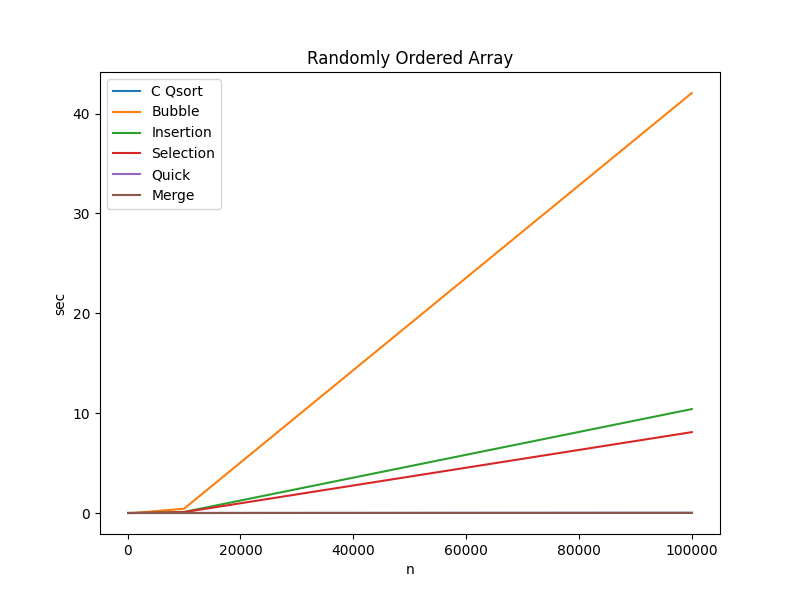
| Algorithm | n=100 | n=1000 | n=10000 | n=100000 |
|---|---|---|---|---|
| C Qsort | 0.000006 sec | 0.000076 sec | 0.000983 sec | 0.013208 sec |
| Bubble | 0.000058 sec | 0.003743 sec | 0.426533 sec | 42.063396 sec |
| Insertion | 0.000013 sec | 0.000995 sec | 0.105663 sec | 10.407530 sec |
| Selection | 0.000013 sec | 0.000878 sec | 0.083730 sec | 8.098650 sec |
| Quick | 0.000006 sec | 0.000080 sec | 0.001028 sec | 0.012784 sec |
| Merge | 0.000006 sec | 0.000080 sec | 0.001083 sec | 0.014232 sec |
Key Takeaways:
- Quick Sort, Merge Sort, and
C’sqsortall perform fairly consistently - Bubble Sort is the worst performer by a wide margin
- Bubble Sort, Insertion Sort, and Selection Sort perform well when $n \leq 10000$; however, the performance degrades exponentially with higher input sizes
Array Sorted in Ascending Order
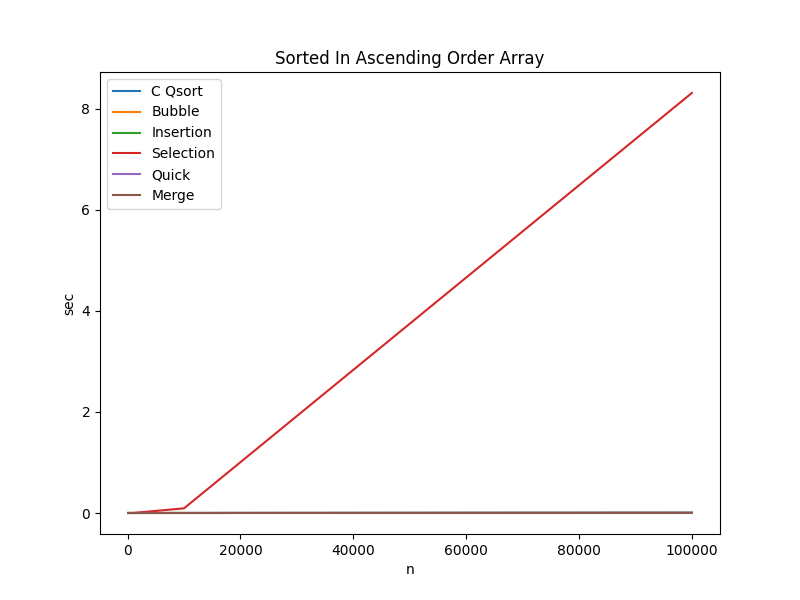
| Algorithm | n=100 | n=1000 | n=10000 | n=100000 |
|---|---|---|---|---|
| C Qsort | 0.000003 sec | 0.000030 sec | 0.000354 sec | 0.004545 sec |
| Bubble | 0.000001 sec | 0.000002 sec | 0.000018 sec | 0.000178 sec |
| Insertion | 0.000003 sec | 0.000019 sec | 0.000183 sec | 0.001822 sec |
| Selection | 0.000011 sec | 0.000893 sec | 0.092301 sec | 8.307492 sec |
| Quick | 0.000003 sec | 0.000028 sec | 0.000324 sec | 0.004177 sec |
| Merge | 0.000003 sec | 0.000032 sec | 0.000433 sec | 0.005164 sec |
Key Takeaways:
- Bubble Sort even outperforms
C qsortwith pre-sorted input data - Insertion Sort is $\approx 4560$ times faster than Selection Sort when $n=100000$ and the input data is pre-sorted
Array Sorted in Descending Order
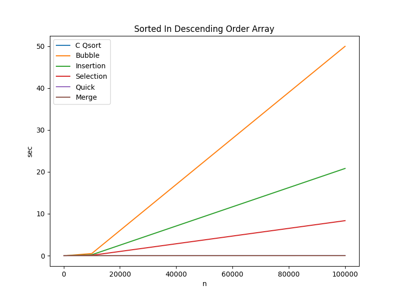
| Algorithm | n=100 | n=1000 | n=10000 | n=100000 |
|---|---|---|---|---|
| C Qsort | 0.000004 sec | 0.000034 sec | 0.000393 sec | 0.004871 sec |
| Bubble | 0.000052 sec | 0.005086 sec | 0.507747 sec | 49.988927 sec |
| Insertion | 0.000023 sec | 0.002074 sec | 0.209936 sec | 20.821724 sec |
| Selection | 0.000011 sec | 0.000832 sec | 0.082854 sec | 8.353472 sec |
| Quick | 0.000004 sec | 0.000039 sec | 0.000417 sec | 0.004868 sec |
| Merge | 0.000004 sec | 0.000036 sec | 0.000436 sec | 0.005036 sec |
Key Takeaways:
- Bubble Sort is $\approx 10260$ times slower than Quick Sort and Merge Sort when $n = 100000$ and the input data is sorted in reverse order
- Selection Sort is $\approx 2.5$ times faster than Insertion Sort when $n=100000$ and the input data is sorted in reverse order
Source Code
Relevant Files:
Click here for details on generating actual run time data
Exercises
- Using the programming language of your choice, collect runtime data from your own sorting algorithm implementations and compare them to the data supplied here.
-
Memory estimates do not include stack space because stacks are not covered in this material ↩
-
Results will vary depending on the hardware and current workload of the machine on which the benchmarks are run. All data was collected using a docker container running on a Surface Book 2 Laptop (Intel Core i7, 16 GB RAM). ↩ ↩2
-
For those interested, here is a link to the GNU C Library qsort implementation https://code.woboq.org/userspace/glibc/stdlib/qsort.c.html ↩