This section serves as an introduction to the most notorious open question in mathematics and computer science: $P \stackrel{?}{=} NP$ (is $P$ equal to $NP$?). The question forms the root of computational complexity theory and has implications on the limits of computability. Is there a class of problems for which efficient solutions do not exist? If $P = NP$, many of humanity’s most difficult problems are solvable and the opposite is true if $P \neq NP$. Most reputable computer scientist believe that $P \neq NP$; however, it has never been conclusively proven despite countless research hours from the world’s greatest minds. As evidence of the problem’s significance, the Clay Mathematics Institute is offering a one million dollar reward for anyone who can resolve it1. The venerable Donald Knuth has agreed to augment the prize money with a live turkey should anyone produce a $P = NP$ proof2.
One might fairly wonder if internalizing an open research question is worth the effort for the majority of software professionals. Consider this: optimization problems typically have an obvious (aka naive) solution that’s easy to implement. More often than not, these algorithms equate to an exhaustive search with an exponential runtime of $O(2^n)$ or worse which renders them impractical for all but the most trivial input sizes. The next obvious step is to design a clever algorithm for reducing algorithmic complexity. The problem is, this quest may be completely in vain. Studying $P \stackrel{?}{=} NP$ provides practitioners with the requisite insight to know when searching for a better algorithm is futile.
Fun Aside
It’s interesting that the grandiose implications of $P \stackrel{?}{=} NP$ have captured the imagination of the public. See the following pop-science examples:
Movies/TV:
- Traveling Salesman
- Series finale of the HBO series Silicon Valley3.
Books:
Comics:
There are undoubtedly more. If you know of any, please leave a comment and they will be promptly added.
Supporting Concepts
$P \stackrel{?}{=} NP$ originated in John Cook’s now famous 1971 paper entitled The Complexity of Theorem Proving Procedures4. The research approach is heavily influenced by the state of the computing and mathematics fields at that time. The aim of this section is to illustrate the supporting concepts with enough fidelity to allow the reader to fully appreciate the question while avoiding mathematical technicalities. In that vain, the explanations may be a bit “hand wavy” at times.
Efficiency
In 1965, Jack Edmonds published a paper entitled Path, Trees, and Flowers. A portion of the work is dedicated to defining the nature of an “efficient” algorithm. While no formal definition can completely capture the intuitive meaning, Mr. Edmonds offers a palatable solution by classifying algorithms based on computation time that is “algebraic”5 in the size of the problem. This paper forms the basis of how the terms tractable, intractable, efficient, and inefficient are used today.
An efficient algorithm is any algorithm that has a polynomial runtime. That is, on inputs of size $n$, the worst-case running time is $O(n^k)$ for some constant $k$. $O(n)$, $O(n\log_2 n)$, and $O(n^3 log_2 n)$ are all considered efficient algorithms. An inefficient algorithm is any algorithm that has an exponential runtime. That is, for inputs of size $n$, they have a runtime of $O(k^n)$ for some constant $k$. $O(3^n)$, $O(n!)$, and $O(0.5^n)$ are all examples of inefficient algorithms. An efficient algorithm is said to be tractable and an inefficient algorithm is said to be intractable.
These strict definitions of efficiency can cause confusion because a runtime of $O(n^{100000})$ is practically inefficient but technically efficient. Likewise, a runtime of $O(1.000000001^n)$ is practically efficient but technically inefficient. For the purposes here, the reader is asked to accept this inconstancy.
Turing Machines
In 1936, long before the conception of an electronic computer, Alan Turing published a seminal paper entitled On Computable Numbers. The paper describes a thought experiment involving a theoretical automatic computing machine which later became known as a Turing machine6. The paper definitively proved that there are limits to what is computable. More than eighty years later, there is still not a known computing model that is more powerful. There are two ilks of Turing machines: deterministic and non-deterministic.
A deterministic Turning machine is essentially an abstract analog for modern day computers. Real-world physical machines have identical capabilities and constraints. Conversely, a non-deterministic machine is an abstract computing model that assumes a type of clairvoyance7 that is not possible to emulate with any known real-world machine.
It’s not at all obvious, but Turing machines are useful for constructing thought experiments and proofs. Proving that an algorithm will exhibit certain properties on a deterministic Turning machine essentially proves how the algorithm will function in the real world. For the purposes at hand, simply remember that a deterministic Turing machine is realistic and a non-deterministic Turing machine is not. The exceptionally curious reader should refer to any textbook on automata theory for more information.
Problems
Consider three types of problems: optimization, search, and decision. It may seem a bit pedantic to formally define these; however, formal classification is a requirement for proofs.
- Optimization Problem: Finds the optimal (e.g. minimum or maximum) solution to a problem. More formally, given an input $x$, output $y$ such that $f(x, y)$ is optimal. For instance, when searching for a minimum value $f(x,y) = \min_{y^\prime} f(x,y^\prime) _{}$.
- Search Problem: Determines if a given value exists. More formally, given an input $x$, output $y$ such that $\psi(x,y)$ is true if $y$ exists. $\psi$ is some boolean property.
- Decision Problems: Returns a $yes$ if some boolean proposition is true. More formally, given an input $x$, output $yes$ if $\psi(x)$ is true. Again, $\psi$ is some boolean property.
Most of the proofs relating to $P$ and $NP$ are formulated on decision problems8. However, it’s typically easy to specify a problem in more than one way. For instance, the well-known Traveling Salesman Problem (TSP) is usually stated as an optimization problem:
TSP as an Optimization Problem
Given a graph $G$ of vertices $V$ connected via nonzero cost edges $E$, find the lowest-cost Hamiltonian circuit
However, the decision version of TSP is computationally equivalent.
TSP as an Decision Problem
Given a graph $G$ and a cost $k$, is there is a Hamiltonian circuit whose cost $\le k$.
It’s important to remember that a formal proof of a decision problem’s complexity automatically extends to the search\optimization versions of the problem. A optimization\search problem is at least as hard as a decision problem. The predilection for decision problems rests on the fact that they are easier to work with while constructing proofs.
Reductions
A common technique mathematicians employ to solve problems is reduction. That is, reducing a problem with an unknown solution to a problem with a known solution. The practice is a rich source of jokes such as:
How many mathematicians does it take to change a light bulb? One: they just give it to three physicists, thus reducing it to a problem that’s already been solved.
Reductions are a principle tool in computational complexity theory. Proving that a problem has a specific complexity does not necessarily require a ground-up proof. Consider this: if problem $Q_1$ is previously proven to have complexity $\sigma$ and problem $Q_2$ is reducible to $Q_1$ in a polynomial number of steps, then $Q_2$ is essentially proven to have complexity $\sigma$. The formal notation for reducibility is $\leq_p$. $X \leq_p Y$ means that $X$ is polynomial-time reducible to $Y$. Stated differently, $Q_1 \leq_p Q_2$ means that a deterministic Turing machine can transform any instance of $Q_2$ into an instance of $Q_1$, using a polynomial number of steps, in such a way that an answer to $Q_2$ is the same as an answer to $Q_1$. This is depicted in the image below.
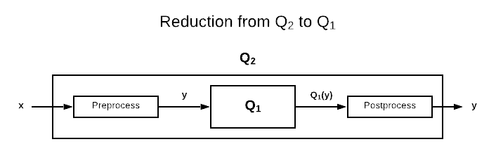
Another way of expressing this concept is to say that if $Q_1 \leq_p Q_2$ then they are the same problem represented in a different language.
With supporting concepts sufficiently defined, the remainder of this work addresses the question straight on.
$P$ or $NP$, That is the Question
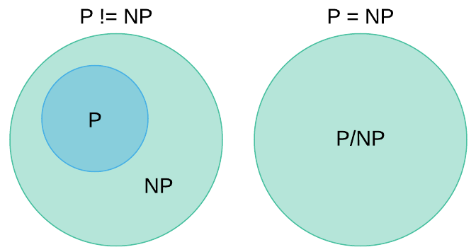
$P$ and $NP$ are complexity classes. Informally defined, a complexity class is a mechanism for classifying problems based on the amount of resources they consume in relation to their input size. The open question is simply: are the complexity classes $P$ and $NP$ equivalent. More accurately, $P$ is known to be a subset of $NP$; however, it is not know if $P$ is a proper subset9 of $NP$ ($P \subseteq NP$). This is depicted in the Venn diagram below.
The complexity class $P$ (Polynomial) contains problems that have efficient solutions. Stated formally, they are decision problems that are solvable by a deterministic Turing machine in polynomial time.
The complexity class $NP$ (Non-Deterministic Polynomial) contains problems that are efficiently verifiable. Efficiently verifiable means that given a particular solution, it’s possible to verify it’s correctness in polynomial time with a deterministic Turing machine10. An efficient verifier is an algorithm with the following characteristics:
- Accepts two arguments: $I$ and $C$ where $I$ is an instance of the problem and $C$ is a certificate that represents a solution.
- Return $yes$ if $C$ is a valid solution.
- Runs in polynomial time given that $C$ is polynomially long.
Because any problem that is efficiently solvable is also efficiently verifiable, all the problems in $P$ are also in $NP$. However, there are many $NP$ problems that have no known tractable algorithmic solution. Stated differently, they are solvable in polynomial time using a non-deterministic Turing machine. Another way to conceive of the difference between $P$ and $NP$ is that $P$ problems can run in polynomial time without providing a certificate ($C$).
To demonstrate, consider the SUBSET-SUM problem: given a set of numbers (\(\{x_1,...,x_n\}\)), does any subset of the numbers sum to exactly $t$. As an example, if \(S = \{1, 2, 3, 4, 5\}\) and $t = 6$. We can ask the question $\langle S, t \rangle \in SUBSET-SUM$. Unfortunately, there is no known efficient algorithm that can answer it. Solving the problem requires a brute force search through all combinations of numbers in $S$. However, given the subset \(\{1, 2, 3\}\), it’s possible to verify its correctness in linear time by adding the numbers together ($1 + 2 + 3 = t$).
To sum $P \stackrel{?}{=} NP$ up, the question is: do problems exist that are efficiently verifiable yet not efficiently solvable? Most computer scientist believe that to be the case; however, no one has been able to conclusively prove it. For all practical intents and purposes, it makes sense to assume $P \neq NP$.
The Hardest $NP$ Problems
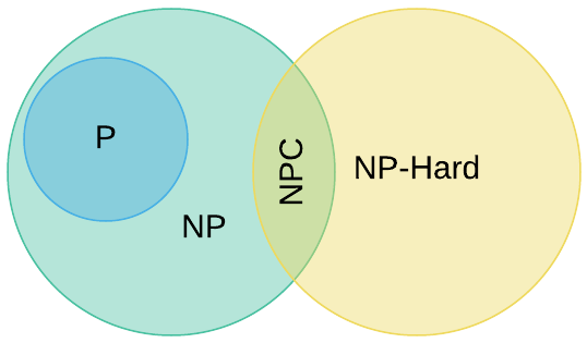
Not all $NP$ problems are created equal11. Assuming $P \neq NP$12, the complexity class $NPC$ (aka $NP$-complete) represents the hardest problems in $NP$. More formally, if a problem resides in $NP$ and every problem in $NP$ is reducible to it ($P^\prime \leq_p P$ for every $P^\prime \in NP$), then the problem is in $NPC$. Intuitively, this means the problem is at least at hard as every other problem in $NP$.
There is also another class of problems for which every problem in $NP$ is reducible to. However, these problems are not in $NP$13. This is the $NP$-hard complexity class. The Venn diagram below depicts the relationship between these complexity classes.
$NPC$ problems are considered intractable as the only known solution algorithms require exponential time. Regardless of how fast hardware becomes, it will never be practical to compute answers to these problems. Consider an algorithm with an $O(2^n)$ runtime. A paltry input size of 100 equates to $1.27 \times 10^{30}$ steps which would take trillions of years to compute even with the world’s fastest super computers.
The first $NPC$ problem was presented by John Cook in his 1971 paper entitled The Complexity of Theorem Proving Procedures. The paper presents a proof that the Boolean satisfiability problem (SAT) is $NP$-complete. Shortly thereafter in 1972, Richard Karp published a paper entitled Reducibility Among Combinatorial Problems. This paper demonstrates that twenty other well-known problems are reducible to SAT and therefore belong in $NPC$. Since then, hundreds of problems have been proven to reside in the $NPC$ and $NP$-hard classes. Chances are, all serious software professionals will encounter $NP$-hard problems during their careers.
The fact that every problem in $NPC$ is reducible to every other problem in $NPC$ has an interesting side effect. In the highly unlikely event that a polynomial-time solution were found for any problem in $NPC$, then every problem in $NP$ has a polynomial-time solution. In other words, it would prove that $P = NP$. Take a moment to consider the gravity of that statement.
Taming $NP$-Hard Problems
Readers most likely have a bleak outlook on $NP$-hard problems at this point. However, discovering that a problem is in $NP$-hard does not mean that brute-force search is the only option. Likewise it does not mean that all instances of the problem are equally hard or that it’s not possible to find answers that are close enough to work in practice. Below are some common techniques for dealing with $NP$-hard problems:
- If the input size is sufficiently small, brute force may be an acceptable solution.
- Solving a real-world case may be easier than the general case. $NP$-complete
problems are only intractable in the worst case, they may be solvable in a
reasonable amount of time for specific cases. Examples include:
- Knapsack Problem with polynomial size capacity
- Weighted Independent Set with path graphs
- 2SAT instead of 3SAT
- Maximum Cut is intractable; however, it’s solvable in linear time via breadth first search if the input is a bipartite graph.
- Vertex Cover when the optimal solution is small
- Solve in exponential time but faster than brute-force search. The runtime is still massive but this approach can put much larger problems within reach.
- Use an approximation algorithm (heuristics) to generate proximate answers.
- Exploit the complexity to your advantage. This is the tact employed by modern cryptography.
Of course, there are $NP$-hard problem instances that are resistant to all the above techniques. Unfortunately, there is no escaping the limits of computability. It may be best to redefine goals to align with more tractable problems.
Get to Work
$P \stackrel{?}{=} NP$ remains an open question; however, it’s reasonable to assume that $P \neq NP$ for all practical intents and purposes. This means that there is a class of problems for which efficient algorithms do not exist. This work serves as little more than a high-level introduction. It barely scratches the surface of computational complexity theory. Readers are strongly encouraged to commit considerable time to further research. The book Computers and Intractability is a great place to start. At a bare minimum, software professionals must be able to identify $NP$-hard problems.
-
https://www.claymath.org/millennium-problems/p-vs-np-problem ↩
-
Donald Knuth made a jest at the end of an ACM SIGACT article:
One final criticism (which applies to all the terms suggested) was stated nicely by Vaughan Pratt: “If the Martians know that P = NP for Turing Machines and they kidnap me, I would lose face calling these problems ‘formidable’!” Yes; if P = NP, there’s no need for any term at all. But I’m willing to risk such an embarrassment, and in fact I’m willing to give a prize of one live turkey to the first person who proves that P = NP
-
A few particularly observant viewers noticed a post-it note labeled $P=NP$ in the Done column of a kanban board. Although, to be particularly pedantic, the characters imply they solved the discreet logarithm problem (DLOG), which is not $NP$-complete. Therefore, it does not necessarily imply that $P=NP$. ↩
-
As with most scientific discoveries, the origins are a bit ambiguous. Steven Cook is typically credited with the formulation of $P \stackrel{?}{=} NP$. However, Kurt Gödel and Leonid Levin also deserve a modicum of recognition.
The world-renowned mathematician Kurt Gödel wrote a personal letter to John von Neumann in 1956 formulating $P \stackrel{?}{=} NP$. His work was never published and was essentially lost until the 1980s. Therefore he is not credited with the discovery.
Leonid Levin, from the former Soviet Union, independently formulated the question around the same time. However, Levin’s contributions weren’t widely publicized in the United States until much later for political reasons. The proff that the Boolean satisfiablity problem is $NP$-complete is often called the Cook-Levin theorom. ↩
-
Big-O notation wasn’t commonly used for algorithmic analysis until the 1970s when it was popularized by Donald Knuth. However, the term “algebraic” in this context has essentially the same meaning. ↩
-
Here is a Hideous Humpback Freak blog post providing a bit more insight into Turing machines: https://hideoushumpbackfreak.com/2015/12/21/Turing-Machine-Simulation.html ↩
-
A non-deterministic Turing machine has the completely unrealistic ability to guess the correct answer given polynomially many options in constant ($O(1)$) time. ↩
-
Pedantic assertions concerning decision problems are not uncommon. While it’s technically correct to say that the optimization version of the traveling salesman problem is not $NP$-complete, it’s a meaningless distinction in practice because the two are computationally equivalent. Most respected computer scientist are comfortable relegating such details to the realm of formal proofs and ignoring the technical discrepancy in common language. ↩
-
A proper subset is a subset that is not equal to the parent set. For instance, if $X$ is a proper subset set of $Y$ then all elements in $X$ are included in $Y$ and $Y$ has at least one element that isn’t included in $X$. ↩
-
Although it’s a bit beyond the scope of this work, this definition isn’t strictly correct. $NP$ is a class of problems where $yes$ answers can be verified efficiently by a deterministic Turing machines. The class co-$NP$ contains problems where $no$ answers can be verified efficiently by a deterministic Turing machine. ↩
-
The complexity class $NPI$ ($NP$-intermediate) contains problems that are somewhere between $P$ and $NPC$. Search for literature on Ladner’s theorem to learn more. ↩
-
In the unlikely event that $P = NP$, the complexity classes noted in this section would all just be $P$. ↩
-
Recall that every problem in $NP$ is a decision problem. The $NP$-hard complexity class does not have this requirement. Additionally, there are many $NP$-hard problems that cannot be efficiently verified. ↩