Matrices

graph LR
    classDef currentPage stroke:#333,stroke-width:4px

	ALG(["fas:fa-trophy Algorithmis fas:fa-trophy "])

	ASY_ANA(["fas:fa-check Asymptotic Analysis#160;"])
    click ASY_ANA "./math-asymptotic-analysis"

    

	MAT_NOT(["fas:fa-check Mathematical Notation#160;"])
    click MAT_NOT "./math-notation"

    

	POL(["fas:fa-check Polynomials #160;"])
    click POL "./math-polynomials"

    

	MAT_FUN(["fas:fa-check Math Functions#160;"])
    click MAT_FUN "./math-functions"

    

	LOG(["fas:fa-check Logarithms#160;"])
    click LOG "./math-logarithms"

    

	COM(["fas:fa-check Combinatorics#160;"])
    click COM "./math-combinatorics"

    

	SET_NOT(["fas:fa-check Set Notation#160;"])
    click SET_NOT "./math-set-notation"

    

	GRA(["fas:fa-check Graphing#160;"])
    click GRA "./math-graphing"

    

	BW(["fas:fa-check Bitwise Logic#160;"])
    click BW "./math-bitwise"

    

	MAT(["fas:fa-check Matrices#160;"])
    click MAT "./math-matrices"

    
      class MAT currentPage
    

	ASY_ANA-->ALG
	BW-->ALG
    MAT-->ALG
    COM & GRA & SET_NOT-->ASY_ANA
    MAT_NOT--> SET_NOT
    POL & LOG--> MAT_FUN
    MAT_FUN--> GRA

Matrices are an indispensable tool for solving linear equations. Anyone employed in the data science field will undoubtedly spend a large portion of their time working with them. Therefore, it’s bittersweet that this material only requires a paltry understanding of them. It’s bitter in the sense that a fun and rewarding deep dive into the subject will have to wait for another time. It’s sweet from the perspective that a short respite from algorithms is sufficient to learn enough about matrices to continue on in that exciting endeavor. In this spirit, this section covers only the four matrix operations required to master this content and makes the simplifying assumption that all operations are executed on matrices of the same size.

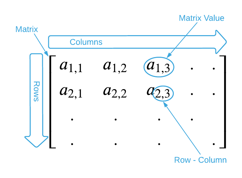
Before jumping right into matrix operations, it’s prudent to define what a matrix is. A matrix is a table of values. Values are arranged by row and column. Every item in a matrix is addressable by it’s row and column number. Consult the image below.

Matrix

PRO TIP: Programmers are quick to point on that the row and column numbers illustrated above are not zero based. This is an unfortunate inconsistency between math and computing literate. However, it’s not a matter for concern. Just remember to adjust the addresses when applying matrices in a computing context.

The height of a matrix is the number of contained rows and the width is the number of contained columns. The height and width together comprise the size of the matrix and is typically denoted as $m \times n$ as shown below.

\[\text{size} = 3 \times 2 \\ \begin{bmatrix} 1 & 2 \\ 3 & 4 \\ 5 & 6 \end{bmatrix} \\ \\ \text{size} = 2 \times 3 \\ \begin{bmatrix} 1 & 2 & 3 \\ 4 & 5 & 6 \end{bmatrix}\]

With the preliminary definitions out of the way, it’s time to dive into the relevant operations: Add, Subtract, Transpose, and Multiply.

$+$ Matrix Addition

Adding two matrices together is a matter of adding together each individual value. This is illustrated below.

\[\begin{bmatrix} 1 & 2 \\ 3 & 4 \end{bmatrix} + \begin{bmatrix} 5 & 6 \\ 7 & 8 \end{bmatrix} \quad = \quad \begin{bmatrix} (1 + 5) & (2 + 6) \\ (3 + 7) & (4 + 8) \end{bmatrix} = \begin{bmatrix} 6 & 8 \\ 10 & 12 \end{bmatrix}\]

$-$ Matrix Subtraction

Matrix subtraction is similar to matrix addition. Simply subtract the corresponding values in the matrices.

\[\begin{bmatrix} 1 & 2 \\ 3 & 4 \end{bmatrix} - \begin{bmatrix} 5 & 6 \\ 7 & 8 \end{bmatrix} \quad = \quad \begin{bmatrix} (1 - 5) & (2 - 6) \\ (3 - 7) & (4 - 8) \end{bmatrix} = \begin{bmatrix} -4 & -4 \\ -4 & -4 \end{bmatrix}\]

$^T$ Matrix Transpose

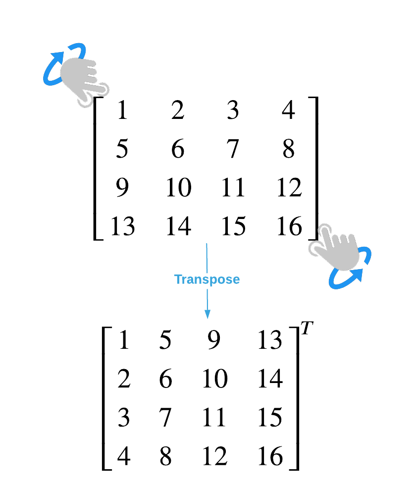
Transpose is typically denoted as $^T$ so that the transpose of $A$ is $A^T$. To transpose a matrix, transform the rows to columns and vice versa. It’s helpful to visualize a transpose operation as grabbing the matrix by it’s corners and flipping it as shown below.

Transpose

Notice how the values running down the diagonal center match between the original matrix and the transposed matrix. This is a useful property that can be exploited algorithmically.

$\times$ Matrix Multiplication

Matrix multiplication is a bit more complicated than the previous three operations. Every value in the result is the dot product of the corresponding row in the first matrix and the corresponding column of the second matrix. The dot product is the sum of the products of the corresponding entities. Consider the example below:

\[A = \begin{bmatrix} 1 & 2 \\ 3 & 4 \end{bmatrix} \quad B = \begin{bmatrix} 5 & 6 \\ 7 & 8 \end{bmatrix} \quad C = \begin{bmatrix} 19 & 22 \\ 43 & 50 \end{bmatrix} \\ A * B = C\]

The value $C_{1,1}$ is the dot product of row 1 in $A$ $(1, 2)$ and column 1 in $B$ $(5, 7)$.

Dot Product

Extending this to all values in the matrix yields:

\[\begin{bmatrix} 1 & 2 \\ 3 & 4 \end{bmatrix} \times \begin{bmatrix} 5 & 6 \\ 7 & 8 \end{bmatrix} \quad = \quad \begin{bmatrix} (1, 2) \cdot (5, 7) & (1, 2) \cdot (6, 8)\\ (3, 4) \cdot (5, 7) & (3, 4) \cdot (6, 8) \end{bmatrix} = \begin{bmatrix} (1 * 5 + 2 * 7) & (1 * 6 + 2 * 8)\\ (3 * 5 + 4 * 7) & (3 * 6 + 4 * 8) \end{bmatrix} = \begin{bmatrix} 19 & 22 \\ 43 & 50 \end{bmatrix}\]

An important thing to note is that, unlike standard arithmetic multiplication, matrix multiplication is not commutative meaning that $A * B \neq B * A$.

Exercises

Assuming that $A = \begin{bmatrix} 8 & 22 & -3 \\ 17 & 28 & 107 \\ -8 & 223 & 138 \end{bmatrix}$ and $B = \begin{bmatrix} 65 & 43 & 54 \\ -48 & 73 & 0 \\ 54 & 756 & -34 \end{bmatrix}$, solve the following problems:
a. $A + B$
b. $A - B$
c. $A^T$
d. $A * B$
Answers (click to expand)
1. $ \begin{bmatrix} 73 & 65 & 51 \\ -31 & 101 & 107 \\ 46 & 979 & 104 \end{bmatrix} $
2. $ \begin{bmatrix} -57 & -21 & -57 \\ 65 & -45 & 107 \\ -62 & -533 & 172 \end{bmatrix} $
3. $ \begin{bmatrix} 8 & 17 & -8 \\ 22 & 28 & 223 \\ -3 & 107 & 138 \end{bmatrix}^T $
4. $ \begin{bmatrix} -698 & -318 & 534 \\ 5539 & 83667 & -2720 \\ -3772 & 120263 & -5124 \end{bmatrix} $