Optimal Binary Search Tree

The Self Balancing Binary Tree section implied that balanced trees provide optimal search run times. This is true given one caveat: the number of searches per item is distributed evenly. If a particular item has a high search frequency it makes sense to place it at the top of the tree. Consider this example:

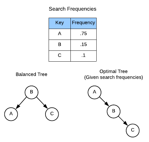
Given the balanced tree, the number of operations to find A and B are 2 and the number of operations to find C is 1. Therefore, the average search time is:

The same calculation on the optimal tree works out as follows:

Over a large number of items, this can add up to many precious processor cycles. The implication is that for scenarios in which the items and their associated search frequencies are known up front, it’s possible to arrange the tree for optimal average search run time.

The other list data structure sections are mainly concerned with calculating the run time of operations. Because binary tree run times are already thoroughly examined, this section focuses on the run time required to generate an optimal binary search tree.

Applications

• List of commonly used application

Asymptotic Complexity

$O(n^2)$

Optimized version = $O(n^2)$

Pseudo Code

inputs:
    input 1
    input 2

side effect(s):
    effect 1
    effect 2

returns:
    some value

invariants:
    1 = 1

// intialize variables

function:
    code here

code goes in here

Source Code

Full Repo

Relevant Files:

• File.h
• File.c
• FileTest.c

Click here for build and run instructions

Advantages

It’s great

Disadvantages

But, it sucks

Actual Run Times

[chart]

[table]