Hash Table

graph LR
	ALG(["fas:fa-trophy Hash Table fas:fa-trophy #160;"])

	ASY_ANA(["fas:fa-check Asymptotic Analysis #160;"])
    click ASY_ANA "./math-asymptotic-analysis"

	ARRAY(["fas:fa-check Array #160;"])
    click ARRAY "./list-data-struct-array"

	LL(["fas:fa-check Linked List #160;"])
    click LL "./list-data-struct-linked-list"

	MF(["fas:fa-check Math Functions #160;"])
    click MF "./math-functions"

	BW(["fas:fa-check Bitwise Logic #160;"])
    click BW "./math-bitwise"

	ASY_ANA-->ALG
	MF-->ALG
	BW-->ALG
    ARRAY-->ALG
    LL-->ALG

All the data structures covered to this point (stack, queue, and priority queue) have organized data to optimize retrieval order. This section expands our algorithmic toolbox to accommodate use cases that require locating data at will using a key value. For instance, consider an address book: a desideratum is to locate any contact by name. That is, locate data in memory using a key. A hash table, aka associative array¹, hash map or dictionary, is perfectly suited to this purpose. What’s even better is that a hash table is capable of storing, deleting, and locating data in constant time ($\Theta(1)$)². Many algorithms can be reduced to repeated lookups; therefore, the ability to perform a search in constant time is invaluable.

History

Hans Peter Luhn, an IBM engineer, is typically credited³ with the discovery of hashing⁴. He released a seminal IBM internal memorandum outlining the concept in 1953. He described placing data into “buckets” and calculating a bucket index by “hashing” a key value. IBM immediately began bringing his idea to fruition. Five years later, IBM rocked the computing world by releasing machines capable of indexing large bodies of text. The achievement made front page news.

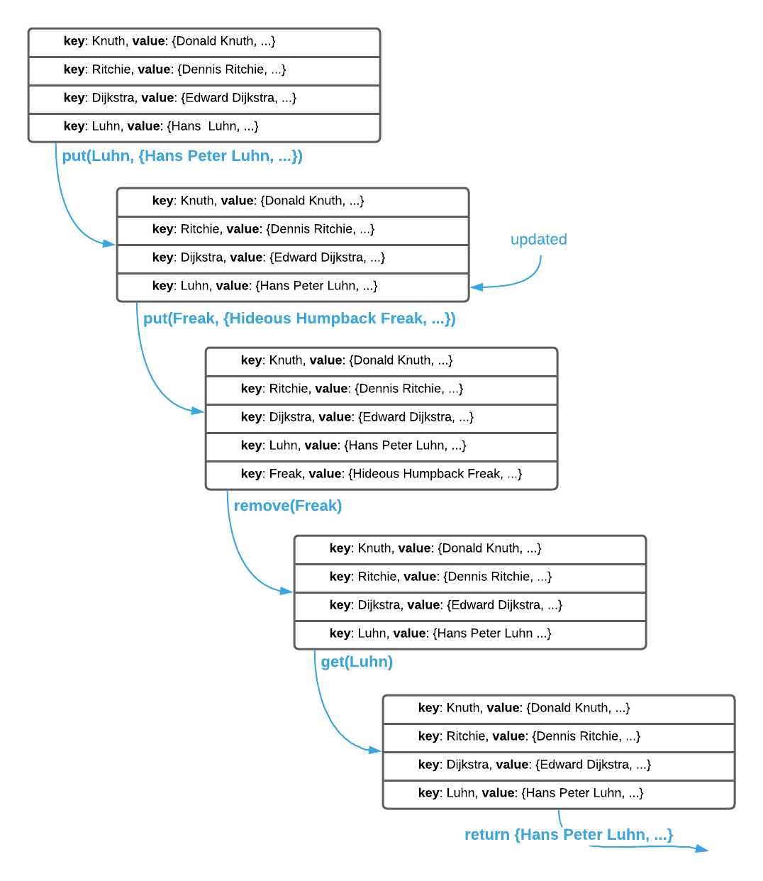
While hash table is an appropriate name given the data structure’s internal workings, dictionary is a more suitable characterization based on the abstract interface. Just like a physical dictionary stores definitions retrievable via a word, hash tables store objects that are retrievable via an arbitrary key. There are three typical operations⁵: put(key, value), get(key), and remove(key). The put operation performs an upsert⁶, get returns the value associated with the supplied key, and remove deletes the key value pair. This is illustrated below.

With a firm grasp on the abstract interface, it’s time to examine the internal workings of hash tables. There are three associated concepts: direct addressing, hashing⁷, and collision management. See the sections below.

Direct Addressing

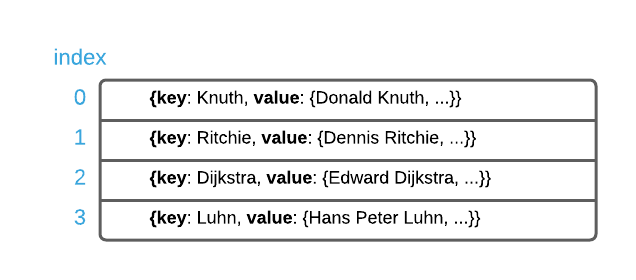
Hash tables store data in arrays. Recall that arrays are contagious segments of memory that support direct addressing. That is to say, assuming a known ordinal index, the memory address of any item is easily calculable in constant ($\Theta(1)$) time. Going back to the example in the previous section, all of the data is stored in an array as shown below.

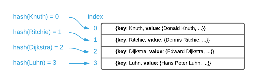
Assuming the knowledge that the key Richie is stored at index 1, it can be retrieved in constant time. Recall from the interface definition that the index is NOT known. The only information available to the algorithm is the key. How is it possible to divine the index given only the key? That’s where hashing comes into play.

Hashing

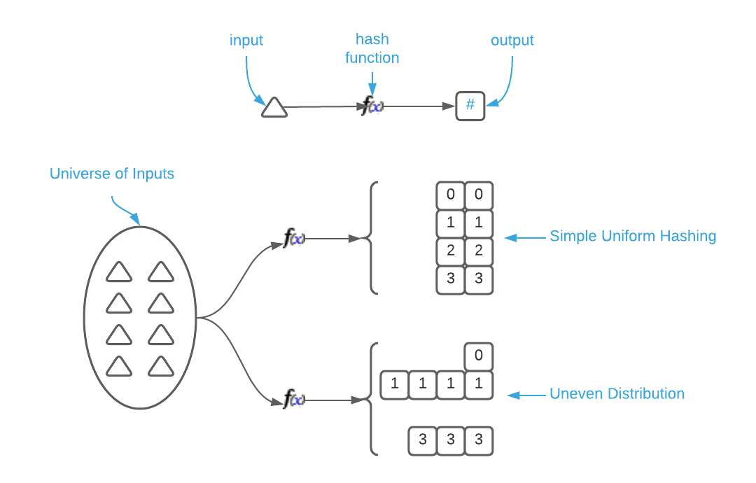
Hashing literally means chop and mix together. A hash function⁸ accepts an arbitrary sized piece of data, chops it up, and commingles it into a fixed length value. In the case of a hash table, the value is an array index. See the image below.

To demonstrate, consider the naive hash function implementation defined in the succeeding pseudo code. There are a couple things to note. The first is that the choice of accepting a byte array is deliberate. Almost any value is convertible to a byte array so this function is capable of generating an index from almost any type of key. The second is that is uses an $\oplus$ (exclusive or aka xor)⁹ to “hash” individual bytes. In a nutshell, $\oplus$ deterministically scrambles the bits.

\begin{algorithm}
\caption{Naive Hash Function}
\begin{algorithmic}
\REQUIRE key = byte array
\REQUIRE bound = array size
\OUTPUT integer $\geq$ 0 and $\lt$ bound
\FUNCTION{hash}{key}
    \STATE hashed $\gets$ key[0]
    \FOR{byte $\in$ key}
        \STATE hashed $\gets$ hashed $\oplus$ byte
    \ENDFOR
    \RETURN hashed $\bmod$ bound
\ENDFUNCTION
\end{algorithmic}
\end{algorithm}

WARNING: Naive hash function is a purely pedagogical device aimed at simplicity. It is not suitable for real-world use.

To summarize, a hash table employs a hash function similar to this one to determine the array index in which to store\retrieve constituent data items. There is however a glaring problem with this implementation. A good hash function has the following proprieties:

1. Efficiently computable.
2. Simple uniform hashing. That is, every output value is equally likely given the input value.

The naive hash function satisfies property one but fails miserably at property two. The return value is derived from a single byte which has a max value of 255; therefore, output values will be clustered in that range. Stated differently, the distribution of output values generated from all possible input values isn’t highly varied. Some indices will occur frequently while others wont occur at all. See the image below.

Another property of simple uniform hashing is that similar inputs must generate widely varied outputs. It’s reasonable to assume that a consumer will store tightly correlated keys in a hash table. It’s important that small key variations generate highly disparate indices. In other words, the keys foo and fop should not produce similar hashes.

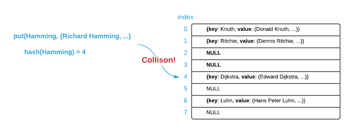
To elucidate the uneven distribution problem, consider a hash table backed by an array of size 8 as depicted below. If the key Hamming hashes to the same index as Dijkstra, they must both somehow be stored at the same index. This is known as a collision. An uneven distribution of keys increases the likelihood of collisions.

Creating a good hash function requires statistics expertise and extensive testing. Luckily, there are several simple and effective non-cryptographic implementations freely available. For instance djb2¹⁰, sbdm, FarmHash, MurmurHash3, and SpookyHash are some popular viable options. Using one of these hash algorithms will probabilistically reduce the likelihood of collisions. The following section explores the possibility of eliminating collisions.

Collisions

Collisions occur anytime a hash function generates the same index for two distinct keys. To create a general-purpose hash table, there are two options:

1. Eliminate collisions
2. Store multiple data items in a single array location

This sub-section explores the first option.

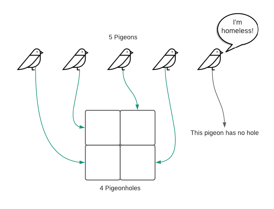
Assuming one knows every possible key in advance and one has access to a sufficiently sized array, it is theoretically possible to eliminate collisions. Unfortunately, such a scenario is exceptionally rare and collisions are otherwise unavoidable. The proof of said fact is demonstrable with a single succinct thought experiment: the pigeonhole principle¹¹. Given $x$ pigeonholes and $x + 1$ pigeons, it’s impossible to place all the pigeons in distinct pigeonholes. See the illustration below.

To demonstrate the relationship to hashing, imagine that an array index is a pigeonhole, a key is a pigeon, and a hash function accepts a pigeon and assigns it to a pigeonhole. Consider a hash table using keys constrained to 10 lower case letters. This equates to $26^{10}$ possible keys. Each key requires a distinct array location. Even if each array item is a mere 16 bytes in size, the total size of the array would be $26^{10} \times 16 \approx 2259 \space \text{terabyte}$. Obviously, this course of action isn’t feasible.

As mentioned in the previous sub-section, it is possible to probabilistically reduce the likelihood of collisions with simple uniform hashing. This is true; however, an actor with intimate knowledge of the employed hashing algorithm can create a pathological data set. A pathological data set is a collection of key values purposefully engineered to prevent even distribution of data. Stated differently, a data set specifically designed to generate a small set of output values given a large set of input values. As the pigeonhole principle illustrates, there will always be multiple input values that generate the same output value. Pathological data is always a possibility¹².

To further exacerbate the collision dilemma, the probability of collisions in unintuitively high even with simple uniform hashing. The concept is best illustrated by the infamous birthday paradox¹³. Suppose there are 367 randomly chosen people in a room. Because there are 365 days in a year, by the pigeonhole principal, there is a 100% probability that two people share the same birthday. This is intuitive; however, the reality that if there are 70 people in the room there is a 99.9% probability of a birthday collision is not so intuitive. In fact, with just 23 people in the room, there is a 50% probability of a collision. The salient point is that if there is a hash table backed by an array of 365 elements, inserting 23 items yields a 50% probability of a collision. Inserting 70 items yields a 99.9% probability of collision.

The bottom line is that it’s theoretically impossible to generate unique indices from keys when the total possible number of keys is larger than the number of indices. Furthermore, the statistical likelihood of collisions is high. The only option is to manage collisions when they inevitably occur.

Chaining

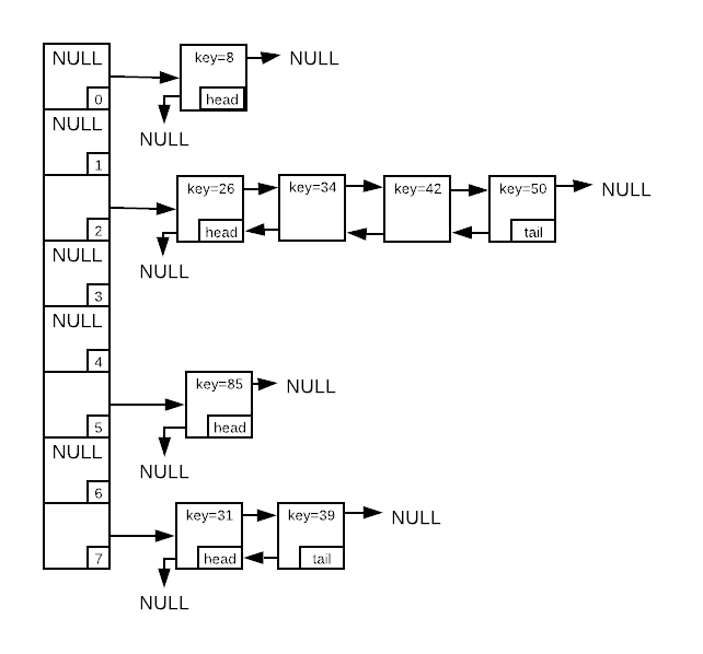
As established, collisions are unavoidable. The only option is to devise a way to map multiple items to a single array index. The most common remedy is chaining¹⁴, which is storing a linked list at each array item. The image below depicts a hash table with integer keys. The array has eight available slots and eight stored items. There were four collisions at index two, so four items are stored in that bucket. Locating an item in the hash table involves generating a hash, locating the desired linked list, and searching it.

The challenge of chaining¹⁵ is that performance degrades as the number of collisions increase. The larger the linked lists becomes, the more searching is required.

Reducing Collisions

There are three implementation details that have impact on collision frequency.

1. Array size
2. Choice of hash function
3. Method to compress hash codes into array indices

They are explored in detail in the sub-sections below.

Array Size

It goes without saying, the larger the array the lower the probability of collisions. A common metric for array sizing is load. Load is the ratio of the count of stored objects to the length of the array. In the chaining image above, the load is $1$ because there are $8$ stored objects and the array has a length of $8$. A rule of thumb is to keep the load below $0.7$. In practice, this means resizing the array and rehashing all the items when the load gets too high. Obviously, this is an expensive operation that should be avoided when possible. Choosing a suitable starting size that balances the cost of resizing with memory consumption is critical.

Choice of Hash Function

Much has already been said about hash functions in the hashing sub-section. Recall that simple uniform hashing reduces the likelihood of collisions so this is the highest concern. There are several freely available hashing algorithms to choose from, all of which have similar characteristics. Choose whichever is most convenient and available for your platform. It’s not recommended to “roll your own” hashing algorithm.

As a final matter of note, hashing functions come in two flavors: cryptographic and non-cryptographic. Cryptographic functions have stronger hashing characteristics but are less performant. It’s recommend to stick with non-cryptographic hashing for hash tables because they are more efficiency computable.

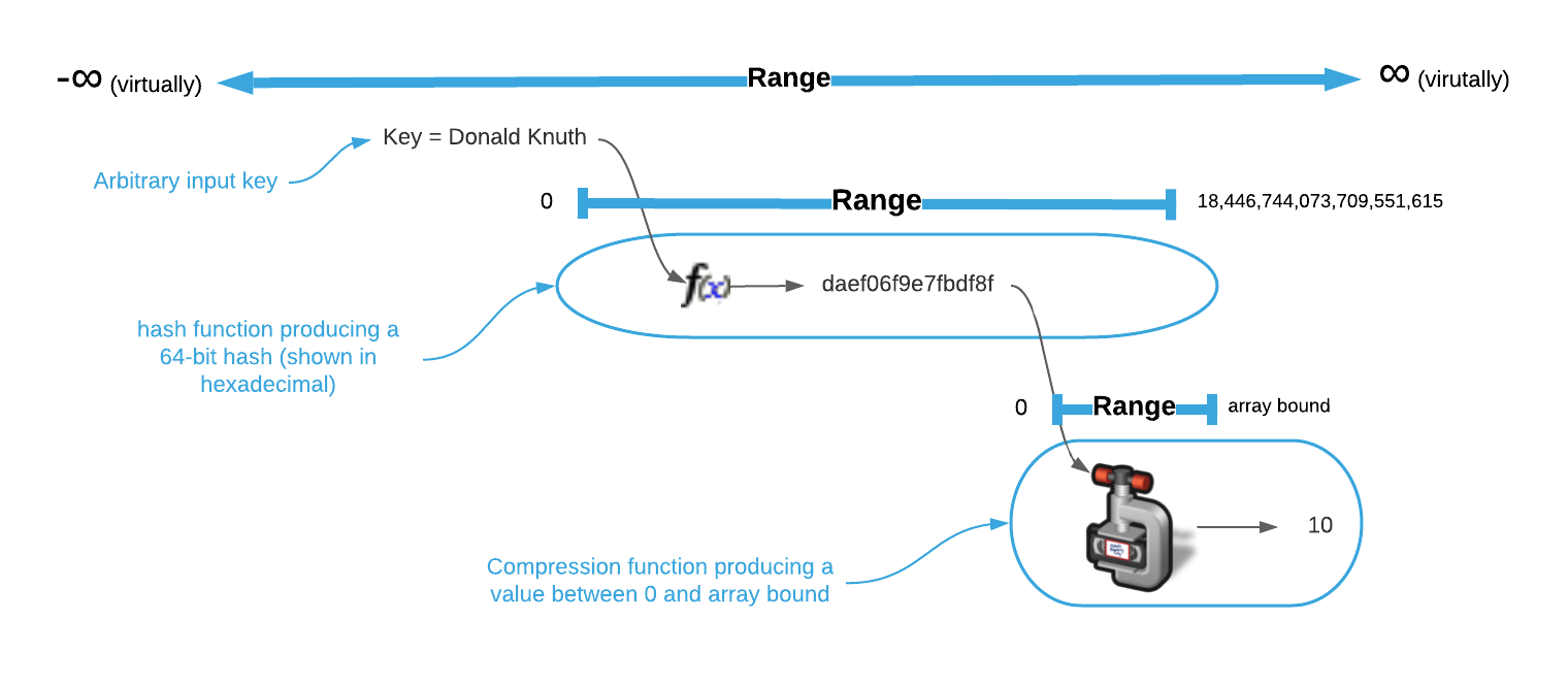
Hash Compression

Hash functions typically return a number with a large range. For instance, FarmHash generates a 64-bit unsigned integer¹⁶ that has a range of $0$ to $18446744073709551615$ inclusive. The hash value must be further compressed into an array bound. This is depicted graphically below.

Compressing a hash value to an array index has implications on the distribution of array indices. There are two common compression techniques: division and multiplication.

The most common reduction method is known as the division method. If $h$ is the hash value and $m$ is the size of the array, the compression formula is $h \bmod m$. This works well is many cases. However, one has to carefully consider the value of $m$. Any common factors between the input keys and $m$ will result in a non-uniform distribution of data. The best way to mitigate this risk to ensure that $m$ has as few factors as possible; therefore, prime numbers are ideal.

The multiplication method is another means of compressing a hash into an array index. It is more complex but has the advantage that the array size is not critical to the distribution of data. The formula for the multiplication method is $\left \lfloor m(hA \bmod 1) \right \rfloor$ where $A$ is a constant, $h$ is the hash value, and $m$ is the array size. The value of $A$ can be anything between 0 and 1; however, Donald Knuth suggests that a good general purpose value is $\frac{\sqrt{5}-1}{2}$¹⁷.

In conclusion, making intelligent decisions for the three most important design considerations will ensure a performant hash table. Unfortunately, there is a great deal of nuance involved that is easy to overlook. Hash tables should not be implemented hastily. Properly implemented, hash tables allow for insertion, deletion, and search in constant time.

Applications

• Countless general purpose programming tasks
• De-Duplication: Inserting items into a hash table automatically removes duplicates by nature of the way they work. This has many applications such as tracking unique visitors to a web site.
• Symbol Tables: Compilers commonly track symbols using hash tables.

Pseudo Code

\begin{algorithm}
\caption{Hash Table Abstract Interface}
\begin{algorithmic}
\REQUIRE key = key to use for future lookups
\REQUIRE value = value to add to the queue
\FUNCTION{put}{key, value}
    \IF{key $\in$ HT}
        \STATE HT[key] $\gets$ value
    \ELSE
        \STATE HT $\gets$ HT $\cup$ (key, value)
    \ENDIF
\ENDFUNCTION
\REQUIRE key = key to search for
\OUTPUT value assoicated with key
\FUNCTION{get}{ht, key}
    \RETURN{HT[key]}
\ENDFUNCTION
\REQUIRE key = key to remove
\FUNCTION{remove}{ht, key}
    \STATE HT $\gets$ HT - (key, value)
\ENDFUNCTION
\end{algorithmic}
\end{algorithm}

Asymptotic Complexity

Assuming a minimal load, non-pathological data, and simple uniform hashing.

• Put: $O(1)$
• Get: $O(1)$
• Remove: $O(1)$

Source Code

Full Repo

Relevant Files:

• hash_table.h
• hash_table.c
• hash_table_test.c

Click here for build and run instructions

Exercises

1. Indicate true of false for each of the following statements.
   a. Simple uniform hashing eliminates collisions.
   b. Simple uniform hashing makes collisions improbable.
   c. Collisions are avoidable.

   Answers (click to expand)

   1. False - Simple uniform hashing reduces the likelihood of collisions.
   2. False - The birthday paradox demonstrates that with 365 possible array indices there is a 50% probability of a collision after just 23 `put` operations.
   3. Either response is acceptable given the perspective.
      True - Strictly speaking, this is theoretically true if you have advanced knowledge of all possible keys and a large enough array. This isn't feasible in practice.
      False - In practice, collisions are not avoidable. The pigeonhole principal provides a simple proof.
      

2. What is the worst case asymptotic complexity for a hash table get operation given the following details:
   • Load $\leq 0.5$
   • Chaining collision management strategy
   • Hash function capable of simple uniform hashing
   Answers (click to expand)

   Linear $O(n)$ - Even with the best designed hash table, it's possible to create a pathological data set that hashes all keys to the same array index. In this case, all items will be stored in a single linked list. The asymptotic complexity of a search operation on a linked list is $O(n)$.
   
   As a matter of note, this scenario is highly unlikely. Such a data set must be deliberately engineered using intimate knowledge of the hash table implementation details.

3. Assume you have a hash table backed by an array of size 50 (indices 0 - 49). Given the hash values below, calculate an array index using both the division and multiplication methods. For the multiplication method, use the constant value of $A = \frac{\sqrt{5}-1}{2}$.
   a. 123456787654321
   b. 243798023461879
   c. 987654321123490
   d. 241378973452560
   e. 246897659028600

   Answers (click to expand)

   1. division = 21
      multiplication = 20
   2. division = 29
      multiplication = 39
   3. division = 40
      multiplication = 7
   4. division = 10
      multiplication = 43
   5. division = 0
      multiplication = 20

4. Specify detailed pseudo code for a hash table implementation with the following characteristics:
   • Consumer specifiable hash function
   • Chaining collision management strategy
   • Multiplication method hash compression

   For formatting purposes, the answers to question 4 are located here.

5. Using the programming language of your choice, create a Least Recently Used (LRU) cache. The abstract interface for the cache is listed below. Assume that all hash table operations are constant ($\Theta(1)$). The requirements are:
   • Asymptotic complexity = $O(\log{n})$
   • Use a hash table
   • Use one of the other data structures covered to this point (stack, queue, or priority queue)
   • Every item must maintain its last accessed time.
   • Every get operation must update the last accessed time of the target item
   • When the cache size exceeds 50, purge the least recently accessed item from the cache
   Answers (click to expand)

   See the C implementation provided in the links below. Your implementation may vary significantly and still be correct.
   - cache.h
   - cache.c
   - cache_test.c

\begin{algorithm}
\caption{LRU Cache Abstract Interface}
\begin{algorithmic}
\REQUIRE key = arbirary key value
\REQUIRE func = function that returns cacheable value
\OUTPUT value associated with key
\FUNCTION{get}{key, func}
    \IF{key $\notin$ C}
        \STATE C[key] $\gets$ func(key)
    \ENDIF
    \STATE C[key].lastAccess $\gets$ now
    \RETURN{C[key]}
\ENDFUNCTION
\end{algorithmic}
\end{algorithm}