Prerequisites (click to view)
graph LR
	ALG(["fas:fa-trophy Quick Select fas:fa-trophy #160;"])

	ASY_ANA(["fas:fa-check Asymptotic Analysis #160;"])
    click ASY_ANA "./math-asymptotic-analysis"

	ARRAY(["fas:fa-check Array #160;"])
    click ARRAY "./list-data-struct-array"

	QS(["fas:fa-check Quick Sort #160;"])
    click QS "./sorting-quick"

	ASY_ANA-->ALG
	ARRAY-->ALG
    QS-->ALG
As alluded to in this section’s introduction, the advantage of studying algorithms is that it endows the learner with critical problem solving acumen. The benefit associated with merely memorizing popular algorithms is diminutive at best. The goal is to develop algorithmic intuition that enables the application of general techniques to many different contexts. In that vein, quick select repurposes the basic structure of the quick sort algorithm to solve a different problem.
History
Sir Charles Antony Richard Hoare, the progenitor of quick sort, also discovered quick select. He published the algorithm in the Communications of the ACM journal in July of 19611.
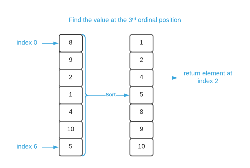
Imagine you have a list of randomly ordered values and you need to identify the element that belongs in the nth ordinal position2. For instance, perhaps you have a list of sporting event scores and you need to determine who came in 3rd place. The obvious solution is to sort the values in ascending order and use Direct Addressing to locate the desired index. For convenience, we’ll refer to this method as sort select. It is depicted in the graphic below.

This is effective, simple, and fairly performant which means that it’s more than adequate for the majority of applications. However, when CPU cycles are at an absolute premium, quick select may be a better choice.
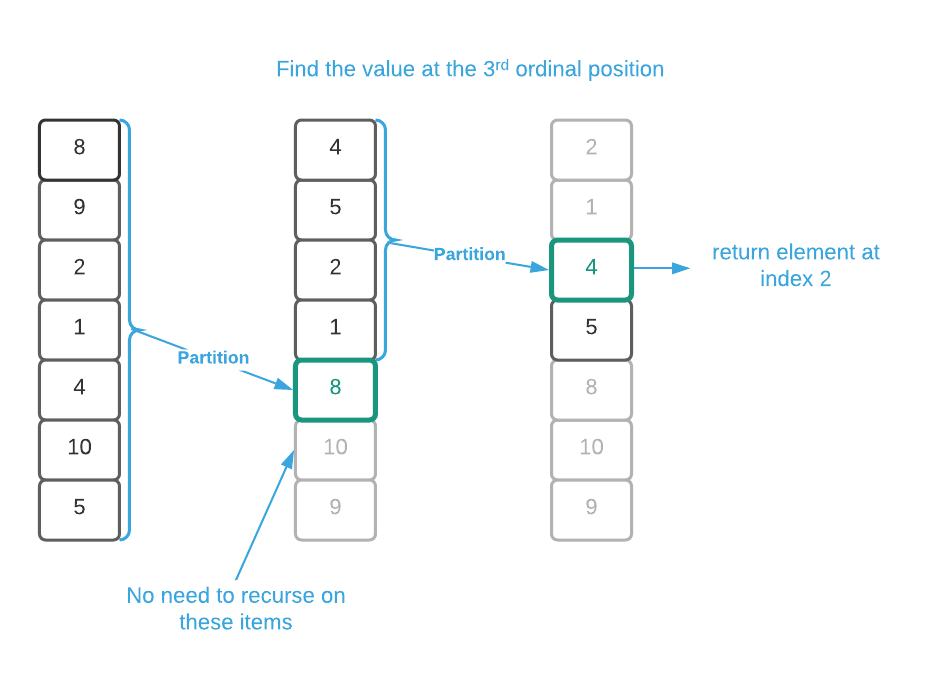
As review, quick sort is a divide and conquer algorithm that’s strictly $O(n^2)$ but $O(n \log_2{n})$ on average. It works by partitioning around a chosen element and recursing on all elements to the left and all elements to the right of the partition. Quick select follows the same basic procedure but it only needs to recurse on either the left or right set of elements. Study the supplied pseudo code in conjunction with the image below to understand how the algorithm works. As a matter of note, the image is depicting a pivot on first choose pivot strategy.

Unfortunately, quick select does not improve on the worst case runtime of quick sort. It’s strictly $O(n^2)$; however, because the number of recursions are essentially reduced by half, the average complexity of quick select is $O(n)$. Based on this, quick select appears to outperform sort select by a factor of $\log_2{n}$ in the average case.
As has been continually trumpeted throughout this material, asymptotic complexity is a single data point among many. The following subsection presents a real-world performance analysis.
Actual Run Times
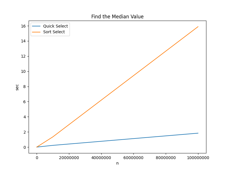
The cardinal rule of performance optimization is always measure. It’s frightfully easy to inadvertently increase run times while attempting to decrease them. The chart and table below contain actual run times for determining the median3 value in an array of integers of size $n$.

| Algorithm | n=100 | n=10000 | n=100000 | n=1000000 | n=10000000 | n=100000000 |
|---|---|---|---|---|---|---|
| Quick Select | 0.000003 sec | 0.000254 sec | 0.002721 sec | 0.020194 sec | 0.224551 sec | 1.833778 sec |
| Sort Select | 0.000004 sec | 0.001039 sec | 0.011118 sec | 0.127531 sec | 1.343921 sec | 15.889618 sec |
Key Takeaways:
- There is $\approx$ 100 milliseconds difference between the two algorithm when $n$ is as high as one million.
- There is $\approx$ 14 seconds difference between the two algorithm when $n$ is as high as one hundred million.
Applications
- Database query engines
- Statistics applications (find median value)
Pseudo Code
\begin{algorithm}
\caption{Quick Select}
\begin{algorithmic}
\REQUIRE $A$ = list of numbers
\REQUIRE $n$ = number of items in input array
\REQUIRE $nth$ = the ordinal position to identify
\REQUIRE
\OUTPUT item from $A$ that
\FUNCTION{quickSelect}{A, n, nth}
    \IF{$n \leq 1$}
        \RETURN $A_0$
    \ENDIF
    \STATE pivot $\gets$ \CALL{choosePivot}{n} \COMMENT{see quick sort for choosePivot implementation}
    \STATE swap $A_0$ and $A_{\text{pivot}}$
    \STATE pivot $\gets$ \CALL{partition}{A} \COMMENT{see quick sort for partition implementation}
    \STATE
    \IF{pivot = nth}
        \RETURN $A_{\text{pivot}}$
    \ELSEIF{nth < pivot}
        \RETURN \CALL{quickSelect}{$A_0...A_{\text{pivot - 1}}$, pivot, nth - pivot}
    \ENDIF
    \STATE pivot $\gets$ pivot + 1
    \STATE \RETURN \CALL{quickSelect}{$A_{\text{pivot}}...A_{\text{n-pivot-1}}$, n - pivot, nth}
\ENDFUNCTION
\end{algorithmic}
\end{algorithm}
Asymptotic Complexity
$O(n^2)$; however, it’s $O(n)$ on average
Source Code
Relevant Files:
Click here for build and run instructions
Exercises
-
Assume you have a list of $\approx$ one million randomly ordered values and you need to identify the top 500 ordinal ranked values. Which algorithm will provide the best performance?
Answers (click to expand)
In this case, sort select is the better choice. Quick select will need to be executed 500 times, one for each desired result (1-500). Conversely, the data only needs to be sorted once to divine all 500 results using direct addressing.
-
What data configuration will force the quick sort algorithm to exhibit the worst case run time ($n^2$).
Answers (click to expand)
If the input data is pre-sorted and the algorithm is using the "pivot on first" choose pivot strategy, the result is the worst case runtime of $n^2$.
- Using the programming language of your choice, implement a quick select
function that accepts:
- an array of any type
- a sorting strategy
Answers (click to expand)
See the C implementation provided in the links below. Your implementation may vary significantly and still be correct.
- quick_select.h
- quick_select.c
- quick_select_test.c -
Using the quick select function created in the previous exercise, determine the median value contained in the sort.txt file.
Answers (click to expand)
See the C implementation provided in the
QuickSelect_find_median_valuefunction located in this file: quick_select_test.c. Your implementation may vary significantly and still be correct. The final output should be:5001.
-
Available online at https://dl.acm.org/doi/10.1145/366622.366647 ↩
-
This is similar to the rank operation introduced in the list data structures section. The only difference is that here we find the item that belongs in the nth ordinal position while rank returns the nth ordinal position of a given element. ↩
-
For the purposes of this project, median is defined as the $\floor{\frac{n}{2}}$th element. Technically, if the number of elements is even, it should be the average of the middle two elements. A somewhat pedantic point, but it may be important in some contexts. ↩