Welcome to the final installment of this three-part series on coding theory. If you have not had the opportunity to read the first two pieces, it is highly recommended that you do before continuing on. They are available here:
- Coding Theory (Part 1 of 3) - Coding Theory Defined
- Coding Theory (Part 2 of 3) - Coding Theory Defined
Having covered cogent concepts in previous posts, this article aims to dive into a demonstration which consists of defining a code using a generator matrix and correcting errors using a parity check matrix. The example is a bit contrived and thoroughly simplified for the sake of brevity. However, the intent is not to provide an exhaustive resource; it is to familiarize the reader with coding theory and hopefully entice him/her into further inquiry.
As a fair warning, this post contains a modest amount of high school/first year college level math. An understanding of Boolean algebra (integer arithmetic modulo two) and matrices are a welcomed asset to readers. However, learners less accustomed to these concepts can still follow along and simply have faith that the math works out as advertised. A cursory overview of relevant math concepts is provided where appropriate.
Generator Matrix
A generator matrix is a simple, yet particularly clever means of generating codes. They are comprised of an identity matrix combined with an arbitrary matrix. Multiplying a message in row matrix form by a generator matrix produces a codeword. This is difficult concept to grasp without an example. Therefore, the remainder of this section is step-by-step instructions for creating a generator matrix that will produce a code with eight codewords.
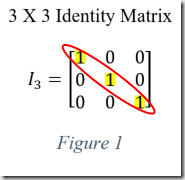
The first step is to define an identity matrix which is a matrix that any given matrix can be multiplied by without changing the value of the given matrix. This is accomplished by setting the principal diagonal elements to one and leaving the rest as zero. See figure one for an example. The matrix is of order three because a three-digit binary string can represent eight possible values which is the number of desired codewords.
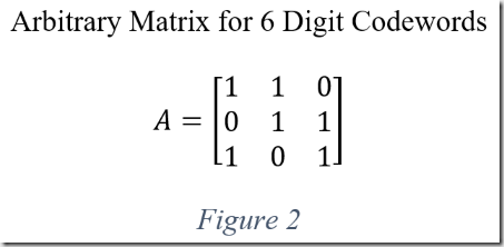
The next step is to define an arbitrary matrix (denoted by \(A\)). The size of the matrix determines the size of generated codewords. If \(m\) is the size of the identity matrix, and \(n\) is the desired length of codewords, then the arbitrary matrix should be of size \(m−by−(n−m)\). Six digit codewords suffice for the purposes of this article; therefore, the arbitrary matrix must be sized three by three (six-digit length minus three-digit identity). Figure two is \(A\) as used by the remaining examples.
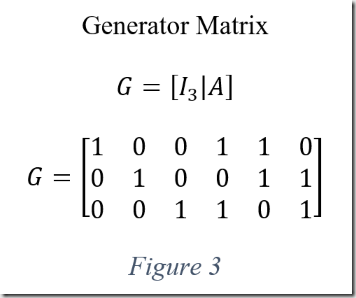
The only thing left do is combine the two matrices above together to form \(G\). It’s as simple as placing them side by side as shown in figure three.
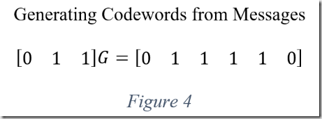
With the generator matrix (\(G\)) in hand, generating codewords is trivial. Multiplying any three-digit binary message in row matrix form produces a codeword. For example, the message \(011\) becomes the codeword \(011110\) as shown in figure four. Notice the codeword is the original message with three parity bits appended. This happens because the generator matrix begins with an identity matrix.
Examining the Code
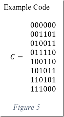
The example code (\(C\)) is comprised of every number between \(000\) and \(111\) multiplied by the generator matrix as shown in figure 5. The example code has a couple of notable attributes. The first is that the sum of any two codewords is yet another codeword. This is known as a linear code. Another extraordinary characteristic is that the minimum hamming distance of the code is equal to the minimum weight of the nonzero codewords. Weight is the number of ones within a codeword. The reasons for this are beyond the scope of this post; it is mentioned to seduce the reader into continued exploration. Examining the code reveals that the minimum hamming distance is three (\(d(C)=3\)).
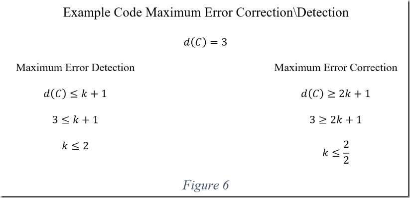
With the code in hand, it’s possible to calculate the equations outlined in part two of this series. First, it’s pertinent to know how many errors the code is capable of detecting and correcting. The previous paragraph defines the minimum hamming distance as three. Figure six demonstrates that the example code is capable of detecting a maximum of two errors and correcting a maximum of one.
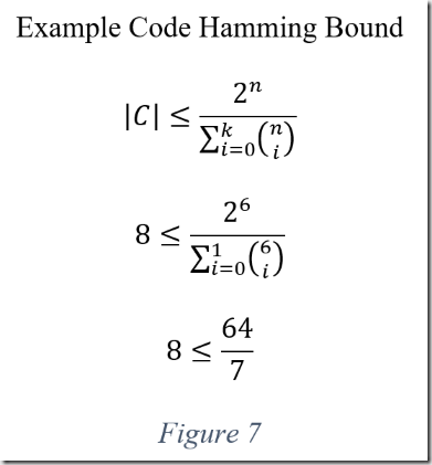
Another relevant equation introduced in the second installment of this series is the Hamming bound. Recall that the \(|C|\) denotes the upper bound number of codewords, \(n\) is the length of the codewords, and \(k\) is the maximum number of errors the code is capable of correcting. Figure seven demonstrates plugging these variables into the Hamming bound equation.
The remainder of this post deals with detecting and correcting errors after transmission. Parity check matrices, described in the next section, are a counterpart to generator matrices that facilitate error detection and correction.
Parity Check Matrices
Parity check matrices are derived from generator matrices. They are used during the decoding process to expose and correct errors introduced during transmission. Multiplying a parity check matrix by the transpose of a codeword exposes errors. The concept is best elucidated by demonstration.
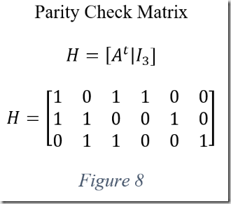
A parity check matrix (denoted as \(H\)) is comprised of the transpose of the arbitrary matrix combined with the identity matrix. As a refresher, the transpose of a matrix is simply the matrix flipped across it’s diagonal so that the \((i,j)\)th element in the matrix becomes the \((j,i)\)th element. Figure 8 shows the parity check matrix that corresponds to the generator matrix from the running example.
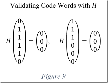
Multiplying the transpose of any valid codeword by the parity check matrix produces a zero-value result as demonstrated in figure nine. The mathematical rational for this this is beyond the scope of this post. However, it is a worthwhile endeavor for the reader to research this further.
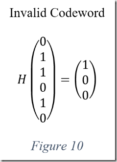
Changing any of the bits in the codeword produces a non-zero result which indicates an error. Consider \(011010\), as shown in figure ten. The result does not equal zero so at least one of the bits is erroneous.
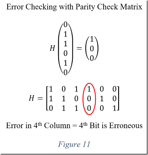
After identifying an inaccurate codeword, it may be possible to correct it using \(H\). Continuing with the example above; the product of the codeword and \(H\) is equal to the forth column in \(H\). This indicates an error in the fourth bit and changing the fourth bit produces the correct codeword. See figure eleven for an illustration.
Because the example code is only capable of correcting a single error, changing more than one bit generates an irrecoverable codeword. However, with a more complex code, it is possible to correct multiple errors using the distinct sum of \(H\) rows and the nearest neighbor method. Again, the reader is encouraged to expand on this with more research.
Conclusion
This concludes the three-part series on coding theory. Coding theory is a fascinating field that enables the reliable transfer of information in spite of the shortcomings inherent in computing machinery. Richard Hamming, a pioneer in the field, devised ingenious codes that allow a maximum amount of data recovery using a minimum amount of redundancy. His codes are still widely used and have many practical applications. This post demonstrated Hamming’s methods by providing step-by-step instruction for generating codewords using a generator matrix. Additionally, it illustrated how to derive a parity check matrix from the generator matrix and use it to correct errors.
Thank you for taking the time to read this series of articles. As always, I’m happy to answer any questions or embellish details in future posts upon request. I hope this series has enthused the reader into more acute exploration.